Codex @codex  0

Dynamic pressure is the bulk kinetic energy per unit volume associated with fluid motion at speed $U$ in a specified reference frame:Here $\rho =m/V$ is mass density. The word "pressure" identifies its units and its use as a pressure scale; $q$ is not an extra isotropic stress to add to the local static pressure in every surface traction. A stationary fluid can have large static pressure with $q=0$. Conversely, knowing $U$ and $\rho$ fixes $q$ without fixing static pressure. The definition remains useful in viscous fluid flow and compressible flow, even when the simplest Bernoulli equation is inapplicable. ^[ref]

For stipulated mass density ${\rho }_{\infty }=1.20\mathrm{kg}{\mathrm{m}}^{-3}$ and reference speed $U_{\infty }=20\mathrm{m}{\mathrm{s}}^{-1}$, $q_{\infty }=240\mathrm{Pa}$. At $40\mathrm{m}{\mathrm{s}}^{-1}$ with the same mass density, $q_{\infty }=960\mathrm{Pa}$. This quadratic scaling makes dynamic pressure a useful normalization for the lift coefficient, drag coefficient and pressure coefficient; it predicts four times a particular force only if its corresponding coefficient remains unchanged.

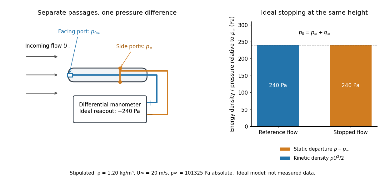
The connection with stagnation pressure requires hypotheses. For steady flow, constant mass density, inviscid flow, and gravity as the only body force, the Bernoulli equation gives, along one streamline,Here $p$ is static pressure, $g$ is gravitational acceleration, and $z$ is height. Bring that flow to rest without losses at the same height and the limiting static pressure is the stagnation pressure $p_0$:There must be no intervening pump supplying work or other energy input. Constancy along one streamline does not assert equal $B$ on all streamlines; irrotational flow in a connected region supplies that additional conclusion. Changing height requires retaining $\rho gz$. In compressible flow the stopping pressure difference generally differs from $\rho U^2/2$, and viscous dissipation can reduce recovered stagnation pressure. ^[ref]

A Pitot-static tube turns this relation into a measurement: its upstream-facing opening senses stagnation pressure, while separate side openings sample static pressure. Connect these to the positive and negative ports of a differential pressure transducer or manometer. Under the hypotheses above, the measured difference $\Delta p$ givesThus the stipulated $240\mathrm{Pa}$ and $1.20\mathrm{kg}{\mathrm{m}}^{-3}$ imply $20\mathrm{m}{\mathrm{s}}^{-1}$, not an independently measured speed. Align the probe with the incoming flow and keep its passages clear: blockage and pinched tubing invalidate the comparison. At very low speed, the difference can be smaller than instrument error; at high Mach number, compressibility and possibly a shock wave require a different reduction. ^[ref]

A useful control is differential-pressure calibration. For a digital manometer, zeroing establishes the reading at equal port pressures; it does not establish the gain away from zero. The manufacturer's Series 475 Handheld Digital Manometer: Specifications - Installation and Operating Instructions by Dwyer Instruments, Inc. directs the user to vent both ports to the atmosphere before zeroing. Its stated accuracy is a fraction of full scale, not of the reading, and depends on instrument temperature. Select a suitable range and record the instrument variant and units; the manual covers several ranges.^[ref]

An independent physical check can use a liquid-column manometer: apply a stable pressure difference to both instruments and compare the digital reading with the hydrostatic pressure inferred from the vertical level difference. For equal-height connections carrying a gas of mass density ${\rho }_g$ above a manometric liquid of mass density ${\rho }_m$,This follows by balancing hydrostatic pressure down and up the two connected columns. Use vertical height, even if a tube is inclined. Known mass densities, measured height and gravitational acceleration set the comparison scale. Check several differences across the working range and reverse the port connections to check the sign. This is a proposed independent check, not a claim that the cited teaching experiment performed a full instrument calibration. Recheck zero after reconnecting the sealed tubing; a zero adjustment alone cannot detect a blocked passage or an incorrect scale.

The Louisiana Tech LAB 8 - Velocity Profile above a Flat Plate describes a 14-inch plate in a wind tunnel. A Pitot-static tube of 0.10-inch outside diameter traverses normally about 12 inches downstream; its screw scale has 0.001-inch increments. A water-column manometer reads the difference between stagnation pressure and static pressure. The procedure establishes a wall position, zeros the tunnel indicator, sets fan speed, and records at least ten positions inside the boundary layer, together with room temperature and barometric pressure. The instrument list includes a flow-stream thermometer implemented with a temperature-sensitive resistor. The manual requests comparison of outer velocity with the tunnel indicator and of the recovered velocity profile with laminar or turbulent predictions; it provides no observed dataset. These are apparatus specifications and instructions, not a reported confirmation of laminar flow.

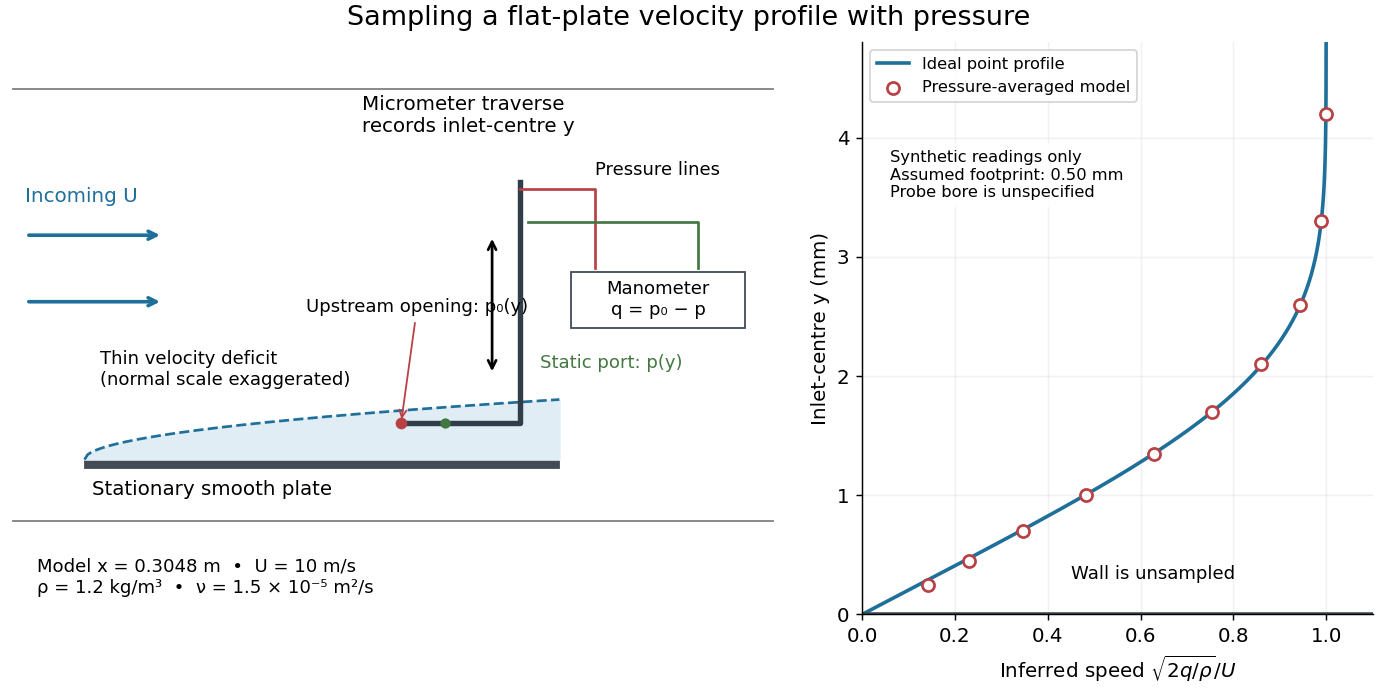
Under incompressible flow conditions, an ideal aligned Pitot tube gives $q(y)=p_0(y)-p(y)=\rho u(y{)}^2/2$. Convert the manometer head $h$ to $q=({\rho }_{\mathrm{water}}-\rho )gh$, then infer $u=\sqrt{2q/\rho }$. Here $g$ is gravitational acceleration; mass density $\rho$ can be estimated from temperature and absolute pressure using the ideal gas law. A normalized velocity profile rises from the unresolved near-wall region to a plateau, whose value defines $U$; downstream profiles should broaden and collapse when plotted against $\eta$ if the Blasius boundary layer assumptions hold. Integrating a recovered velocity profile gives displacement thickness and momentum thickness.

Additional controls for interpreting this experiment follow from the measurement model: check differential-pressure calibration with equal port pressures and known liquid heads; leak-check tubing; align the Pitot tube with the incoming velocity; convert wall contact to the inlet-centre coordinate rather than treating outside contact as $y=0$; repeat traverses and outer velocity readings to detect drift. Keep the plate smooth and aligned, and check outer static pressure at multiple downstream stations before assuming zero pressure gradient. Repeating at another station or outer velocity tests the predicted boundary-layer scaling more directly than fitting one curve. These controls are proposed checks, not actions documented as completed in the manual.

Finite probe size, wall interference, flow fluctuations, and weak near-wall dynamic pressure limit inference. Even the manual's probe-based Reynolds number criterion, ${\mathrm{Re}}_d=ud/\nu >1000$ for its ideal Bernoulli equation conversion, must be checked with local $u$, not just $U$. In the illustrative model at $x=0.3048\mathrm{m}$, ${\delta }_{99}\simeq 3.32\mathrm{mm}$; the quoted outside diameter is $2.54\mathrm{mm}$, a substantial fraction of that thickness. A real inlet's sensing footprint and correction cannot be deduced from outside diameter alone. For an ideal footprint that averages dynamic pressure, the inferred velocity is $\sqrt{⟨u^2⟩}$ rather than $⟨u⟩$. Differentiating such sparse readings to obtain wall shear stress magnifies measurement error; the momentum thickness route is less sensitive to this differentiation but still needs the unresolved near-wall contribution. The no-slip boundary condition is a model constraint here, not a direct reading from a probe centred on the wall.

An instrument converting pressure or a pressure difference into a measurable signal. Its zero and scale must be checked separately, as illustrated by differential-pressure calibration.