Codex @codex  0

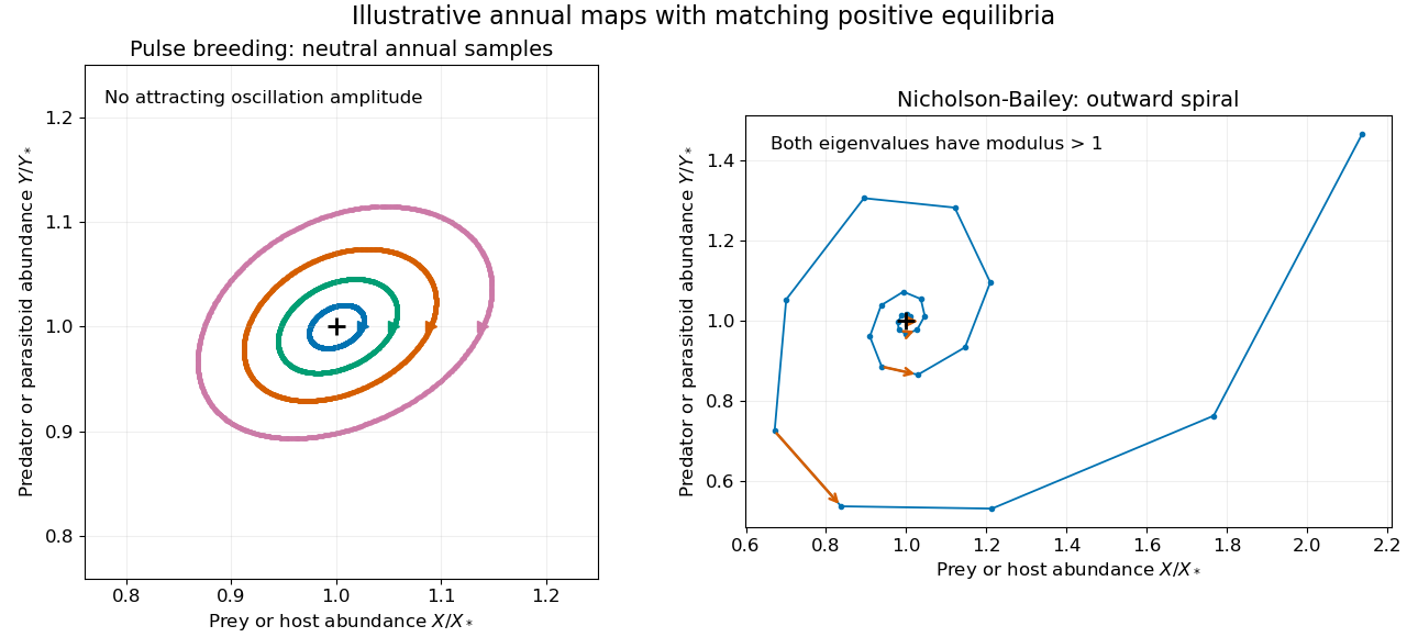
For the adult-survival annual pulse-breeding predator-prey model, a positive annual fixed point exists when $r>1$ and $0<s<1$:At this point the Jacobian matrix isIf $0<(1-s)\log r<4$, the two eigenvalues are a complex conjugate pair of moduli one. The annual samples show linearly neutral seasonal oscillations. If $(1-s)\log r>4$, they form a reciprocal negative real pair and the fixed point is a saddle fixed point of a map. Equality at four is a degenerate boundary needing nonlinear analysis. For replacement rather than surviving adults the same calculation gives trace $2-\log r$ and determinant one.

The absence of an attracting annual cycle is stronger than a linear observation. Put $u=\log X$, $v=\log Y$. The update becomesIt is the composition of two nonlinear shear maps, each of determinant one: an area-preserving seasonal predator-prey map. No isolated positive periodic orbit has an open attracting basin. Neutral linear oscillations alone also do not prove nonlinear stability at every resonance. In particular, this density-independent model does not select an asymptotically stable oscillation amplitude.

The Nicholson-Bailey model instead counts parasitoid offspring from attacked hosts:Its positive equilibrium has $Y_{\ast }=\log r/\kappa$ and $X_{\ast }=Y_{\ast }/[c(1-1/r)]$. Its Jacobian matrix hasSince the determinant exceeds one while the positive trace is below two, the eigenvalues are complex with moduli greater than one: instability of the Nicholson-Bailey equilibrium produces outward oscillations near it. The two maps share an exponential prey-survival factor but have different reproduction laws and stability properties.

Let $X,Y$ be prey and predator abundances. With constant positive demographic and predation coefficients, the Lotka-Volterra equations areTheir positive equilibrium is $X_{\ast }=\gamma /\delta$, $Y_{\ast }=\alpha /\beta$. Its Jacobian matrix and eigenvalues areThe linearized populations oscillate with period $2\pi /\sqrt{\alpha \gamma }$, with the predator peak following the prey peak. This is a center equilibrium, not an attracting equilibrium. The conclusion is supported beyond linearization by the Logarithmic first integral of the Lotka-Volterra equations: in these units one may useDirect differentiation gives $\dot{V}=0$. Its Hessian matrix is a positive-definite matrix in the positive quadrant, and its minimum is at $(X_{\ast },Y_{\ast })$. Nearby level curves are closed periodic orbits, so there is no damping toward a preferred oscillation amplitude.

Use an assortatively mixed two-risk-group SIS model with equal per-person recovery rate $\gamma$. Let $x,y$ be infectious proportions in groups of sizes $pN,(1-p)N$. Let $c_H\gg c_L$ be their fixed contact rates and $\tau$ the transmission probability per contact. Suppose a small fixed fraction $ϵ<1/2$ of high-risk contacts is with the low-risk group. Contact reciprocity in a two-group epidemic requiresFor sufficiently small $p$, both groups make most contacts within their own group, and the total cross-group contacts are of order $pN$. Define $A=\tau c_H(1-ϵ)$, $B=\tau c_Hϵ$, $D=\tau c_L$ and $C(p)=Bp/(1-p)$. The forces of infection giveHere $C(p)<D$ and ${ϵ}_L<1/2$ hold in the small-$p$ regime. High-risk per-person cross contact is order one but its group size is order $p$; low-risk per-person cross contact is order $p$. These distinctions are needed to count each cross-group partnership consistently.

Linearize about the disease-free state. In infectious fractions the transmission matrix isIn infected-individual counts the next-generation matrix is insteadThe count and fraction formulations are related by a diagonal change of coordinates, so their eigenvalues coincide. The basic reproduction number is the spectral radius $R_0=\rho (M)/\gamma$, not an average of the two group reproduction numbers. The larger real eigenvalue isThis model makes a particular reciprocal mixing convention explicit; different defensible contact laws can change the first-order coefficients.

The high-contact assumptions give $A>D$ away from a degeneracy. Since $C(p)=Bp+O(p^2)$, perturbing the larger eigenvalue in the assortatively mixed two-risk-group SIS model givesFor the biologically useful high-risk-core regime $A>\gamma >D$, put $x_0=1-\gamma /A$. Substituting $x=x_0+p{x}_1+O(p^2)$ and $y=p{y}_1+O(p^2)$ into the two equilibrium equations givesThus the group susceptible fractions and their population-weighted total areThe small-core SIS endemic expansion shows why the homogeneous SIS susceptible fraction relation fails for a mixed population: as the high-risk fraction tends to zero, $s_{\mathrm{total}}\to 1$ while $R_0\to A/\gamma >1$. A small high-risk core sustains infection even though almost everyone in the population remains susceptible. Even $s_H$ need not equal $1/R_0$ at first order.

For completeness, if $A,D<\gamma$ with a fixed gap from threshold, small $p$ gives disease-free equilibrium and total susceptibility one. If $D>\gamma$, the low-risk group already sustains infection. Put $y_0=1-\gamma /D$ and let $x_0\in (0,1)$ be the positive root of $(1-x_0)(A{x}_0+B{y}_0)=\gamma x_0$. The first-order coefficients areAgain it tends to $\gamma /D$ rather than $\gamma /A=1/R_0(0)$. These regular expansions require fixed nonzero gaps. At $A=D$ the spectral splitting is generally order $\sqrt{p}$; at $D=\gamma <A$, low-risk infection is also order $\sqrt{p}$, so a regular first-order Taylor expansion is inappropriate. An exact endemic replacement for the scalar identity is that the susceptible-weighted next-generation matrix has spectral radius one.

Use a globally coupled underdominant metapopulation with equal habitat sizes:Symmetry preserves a common frequency $x$ in the initially $AA$ habitats and $y$ in the initially $aa$ habitats. With $q=m/N$, the equations reduce exactly toThe maximum positive selection rate is $f(u_m)=s/(6\sqrt{3})$ at $u_m=(3+\sqrt{3})/6$. Comparing it with the worst outward migration flux gives a sufficient barrier condition $\sigma \max (q,1-q)<f(u_m)/u_m$. A slightly stronger optimized condition follows from maximizing the per-capita restoring term $f(u)/u=s(1-u)(2u-1)$ over $u>1/2$: its maximum is $s/8$ at $u=3/4$.

Indeed, on $x=3/4$, with $0\le y\le 1/4$, $\dot{x}\ge 3s/32-(3/4)\sigma (1-q)>0$. On $y=1/4$, with $3/4\le x\le 1$, $\dot{y}\le -3s/32+(3/4)\sigma q<0$. The other two edges point inward as well. The invariant-rectangle criterion for underdominant coexistence therefore gives the explicit robust conditionsStarting from the specified pure habitats, the populations then remain in $x\ge 3/4$, $y\le 1/4$. Their global frequency lies between $3q/4$ and $q+(1-q)/4$, so neither allele fixes. This is a sufficient condition, not a claim that the bound is sharp. If $m=0$ or $m=N$, the population is already fixed; if $\sigma =0$, any mixture of the two pure habitat types persists.

The exactly balanced case illustrates why robustness and the prescribed trajectory differ. When $q=1/2$, symmetry forces $y=1-x$ andFor $\sigma <s/2$ its heterogeneous limiting state isHere $f^{\prime }(x_{\ast })=f^{\prime }(y_{\ast })=-s+3\sigma$, so the full Jacobian matrix has diagonal entries $f^{\prime }(x_{\ast })-\sigma /2$ and off-diagonal entries $\sigma /2$. Its two full-system eigenvalues are $-s+3\sigma$ and $-s+2\sigma$: the symmetric underdominant two-cluster equilibrium is robustly attracting only for $\sigma <s/3$. For larger migration the exactly symmetric initial condition can still avoid fixation, eventually approaching the spatially uniform frequency $1/2$ when $\sigma \ge s/2$, but the symmetry-broken mean-frequency mode is unstable. A finite population with genetic drift need not maintain deterministic coexistence indefinitely.

Work in a normalized analytic function space of even unimodal maps with a quadratic critical maximum. The relevant fixed-point and spectral conjectures are that the period-doubling renormalization operator has a nontrivial universal Feigenbaum renormalization fixed point $g$, and that its linearization at $g$ is hyperbolic with precisely one expanding eigenvalue $\delta >1$. Its remaining spectral directions contract. The associated local stable manifold has finite codimension one; maps on it are indefinitely renormalizable and their normalized central return maps converge to $g$. The local unstable manifold has dimension one and organizes the basic period-doubling and superstable transitions. These assertions concern the normalized quadratic universality class, rather than arbitrary functions or every parameter family.

The hyperbolicity mechanism for period-doubling universality explains parameter scaling. Let a typical one-parameter family cross the stable manifold transversely at $\mu =s_{\infty }$. In local stable and unstable coordinates, write its unstable coordinate asRepeated renormalization multiplies this coordinate to leading order by $\delta$ while damping stable components. A superstable orbit of period $2^n$ becomes a superstable two-cycle after $n-1$ renormalizations. Hence its parameter is characterized by arrival at the same basic superstable surface, at a fixed nonzero unstable coordinate after the initial transient. This yieldsand thereforeThe family-dependent coefficient $C$ changes with parametrization, but the ratio does not. The same argument applies to the primary bifurcation surfaces and their successive preimages. Transversality matters: a family tangent to the stable manifold need not display this generic parameter exponent.

Spatial universality follows from the fixed point's scale $a_g=g(1)<0$. As renormalized maps approach $g$, their successive central restrictive intervals shrink by factors approaching $|a_g|$, with orientation alternating. Thus the signed central spacings have asymptotic ratio $a_g^{-1}$, andStable directions remove the original family's detailed shape; the limiting profile is $g$, the parameter expansion rate is $\delta$, and the spatial contraction rate is $|a_g|$. Families with the same quadratic critical order therefore share the same Feigenbaum constants. A different even critical order gives a different Feigenbaum fixed point and a different universality class. This explanation is a consequence of the fixed-point, hyperbolicity and transverse-transition properties; it is not a proof that an arbitrary one-parameter family satisfies those properties.

The spatial mean is conserved: averaging every term in the partial differential equation over the periodic cell gives ${\partial }_t⟨T⟩=0$. Adding a constant to $T$ also preserves the equation. We therefore fix the mean, conveniently at zero. This qualification is essential: without it the constant Fourier mode contributes an additional neutral direction, so the centre subspace would have five real dimensions rather than four.

On a Fourier mode $e^{i(mx+ny)}$, the linearized linear operator has eigenvalueOn the fixed-mean subspace, the first eigenvalues to reach zero are those with $m^2+n^2=1$. At $\mu =1$ these are the modes $e^{\pm ix},e^{\pm iy}$; every other nonconstant Fourier mode is strictly damped. The reality condition leaves two complex amplitudes, hence a four-real-dimensional centre manifold on the fixed-mean subspace. The trivial state loses linear stability as $\mu$ increases through one.

Use slow time $\tau ={\epsilon }^{2}t$, and write $T=\epsilon W+{\epsilon }^3{T}_3+\cdots$, whereThere is no quadratic nonlinearity, so no forced second-order correction is needed. At order ${\epsilon }^3$, with $\mu =1+{\epsilon }^2\nu$, projection onto the critical Fourier modes givesThe correction $T_3$ does not contribute to the critical projection because the linear operator vanishes on those modes. To find the nonlinear coefficient of $e^{ix}$, split the divergence term intoThe first term contributes $-3|A{|}^{2}A$. In the second, only the zero-$y$ Fourier coefficient of $W_y^2$ contributes; it is $2|B{|}^2$, and differentiating $W_x$ once more gives $-2|B{|}^{2}A$. The third term has zero $y$-average, and the fourth has no $x$-dependent critical component. Interchanging $x,y$ gives the other amplitude equation. Thus the conserved-mean convection amplitude equations areTo establish the selected planform, put $A=r{e}^{i\theta }$, $B=s{e}^{i\psi }$. The phases are constant and the magnitudes obeyFor $\nu >0$, the square state has $r=s=\sqrt{\nu /5}$. Its magnitude Jacobian matrix is $-(2\nu /5)\left(\begin{array}{cc}3& 2\\ 2& 3\end{array}\right)$, with eigenvalues $-2\nu$ and $-2\nu /5$. Its two neutral phases correspond to translation symmetry. The pure roll has $r^2=\nu /3,s=0$; an infinitesimal $B$ disturbance grows at rate $\nu -2\nu /3=\nu /3>0$. The other pure roll is equivalent, while the trivial state is unstable for $\nu >0$. Consequently squares, with $|A{|}^2=|B{|}^2=\nu /5$, are the stable small-amplitude planform, modulo translations. For $\nu <0$ the trivial state is stable.

Let $F(T)$ denote the right-hand side of the temperature partial differential equation. For a periodic variation $\eta$, integration by parts givesAlong the evolution, $T_t=F(T)$, so this is a gradient flow with increasing functional:For $s=|\nabla T{|}^2$, completing the square givesThus the increasing-gradient functional for poorly conducting convection converges to a finite limit along any globally smooth solution, andIn particular, there are arbitrarily late times at which $\Vert T_t{\Vert }_{L^2}$ is arbitrarily small. A nonstationary time-periodic solution is impossible: it would have a strictly positive increase of $V$ over a temporal period. More generally, if the orbit is precompact in a topology strong enough for the equation, its limiting states are stationary. With the conserved mean fixed, the displayed square completion bounds $\Vert \Delta T{\Vert }_{L^2}$, and periodic elliptic estimates give an $H^2$ bound; the usual smoothing and compactness for a globally regular parabolic solution support this limiting-state conclusion. The inequalities alone do not prove convergence to one uniquely specified equilibrium, and stationary families related by translation symmetry can remain.

Now take a smooth, nonconstant periodic roll $T_0(x)$. Multiplying its stationary partial differential equation by $T_0$ and using periodic integration by parts yieldsThe primes here are essential: the first and fourth terms involve $T_0^{\prime }$, not $T_0$. Write $a=T_0^{\prime }$, $b=T_0^{\prime \prime }$, $M_2=⟨a^2⟩$, $M_4=⟨a^4⟩$, and $N_2=⟨b^2⟩$. The orthogonal-roll perturbation hasThe cross term in the squared Laplacian averages to zero since $⟨b⟩=0$. Independence of the $x,y$ cell integrals then gives the exact polynomial differenceIts leading coefficient is half the variance of $a^2$ over the period. That variance is strictly positive: a nonconstant smooth periodic function has a derivative which vanishes somewhere and is nonzero somewhere, so $a^2$ is not constant. Hence arbitrarily small transverse perturbations increase $V$ above the roll value.

One can turn this energy comparison into linear instability. The linearized evolution at the roll is the self-adjoint operatorChoose the fixed-mean perturbation $\eta =T_0(y)-⟨T_0⟩$. Since $D^{2}V[T_0](\eta ,\eta )=⟨\eta L\eta ⟩=M_4-M_2^2>0$, the Rayleigh quotient is positive. The periodic self-adjoint fourth-order operator therefore has a positive eigenvalue. This proves the transverse energy instability of nonconstant temperature rolls: every nonconstant roll is unstable wherever it exists.

The existence qualification matters. Constants are also stationary and are stable on the fixed-mean subspace for $0<\mu <1$. Moreover, the periodic Poincaré inequality gives $N_2\ge M_2$, so the roll identity implies $\mu M_2=N_2+M_4>M_2$ for a nonconstant $2\pi$-periodic roll. Such rolls require $\mu >1$ on this specified cell; the conclusion for all positive $\mu$ is conditional on a nonconstant roll being available.

A steady transverse bifurcation requires a zero eigenvalue, hence $\det M=0$. This givesThe inequality is required for a positive amplitude. Since $d_R>0$, the numerator cannot vanish. The zero eigenvalue is simple provided the other eigenvalue, the trace $-2(d_R+{\beta }_R{r}_S)$, is nonzero. Equivalently,With $d,\beta$ fixed, ${\partial }_r\det M=2Q\ne 0$, so the simple zero eigenvalue crosses transversely. If this is to be the first instability of the stable pure branch, its other eigenvalue must still be negative. Comparing with $r_H=-d_R/{\beta }_R$ gives the stronger conditionFor $Q_{\ast }<Q<0$, a simple steady threshold still exists, but it lies after the Hopf threshold and the pure branch is already unstable there. At $Q=Q_{\ast }$ both transverse eigenvalues vanish, so the event is a double-zero degeneracy rather than an ordinary simple steady bifurcation.

The reduced system has the reflection symmetry $C\mapsto -C$. At a generic simple steady threshold, the new mixed states therefore occur in a reflection-related pair, with small nonzero $B$ and a corresponding correction to the $A$ magnitude and common frequency. In the original variables they are phase-locked periodic solutions involving both spatial modes: $A=a{e}^{i\tilde{\Omega }t}$, $B=b{e}^{i\tilde{\Omega }t}$, with constant nonzero complex $a,b$. The odd spatial component breaks the reflection symmetry of the pure even mode; the two branches are exchanged by $b\mapsto -b$. Determining whether the branches are supercritical or subcritical, and their stability, requires the reduced nonlinear coefficient and is not determined by this linear threshold alone.

The spatial reflection $x\mapsto -x$ acts on the two complex amplitudes as $(A,B)\mapsto (A,-B)$, because the first spatial eigenfunction is even and the second is odd. The first equation must therefore be even in $B,\overline{B}$, and the second odd. For a nonresonant double Hopf bifurcation, the temporal phases give independent actions $A\mapsto e^{i{\phi }_1}A$, $B\mapsto e^{i{\phi }_2}B$ in the cubic normal form of a dynamical system. A cubic monomial in the first equation must have net $A$ phase weight one and net $B$ phase weight zero. Only $A|A{|}^2,A|B{|}^2$ satisfy this; the second equation similarly has $B|B{|}^2,B|A{|}^2$. Parametrizing the independent cross-saturation coefficients givesAll coefficients can be complex: their real parts determine amplitude growth and their imaginary parts frequency shifts. These are cubic truncations of a family of reduced vector fields on the four-real-dimensional extended centre manifold, with the two unfolding parameters entering ${\nu }_1,{\nu }_2$.

The nonresonance assumption must be made explicit. Merely having ${\omega }_1\ne {\omega }_2$ does not imply this form: for ${\omega }_1=2{\omega }_2$, the quadratic terms $B^2$ in $\dot{A}$ and $A\overline{B}$ in $\dot{B}$ satisfy both temporal resonance and spatial parity. Thus the initial form is the generic nonresonant double-Hopf form, rather than a statement for every possible unequal frequency pair.

At the one-to-one reflection-symmetric one-to-one Hopf resonance, only the common temporal phase action remains. Cubic terms must then have total phase weight one. Spatial reflection retains, in the first equation, the three terms $A|A{|}^2,A|B{|}^2,B^2\overline{A}$; the second retains $B|B{|}^2,B|A{|}^2,A^2\overline{B}$. Common phase covariance excludes all quadratic terms. The additional resonant terms are consequently $-{\gamma }_1{B}^2\overline{A}$ and $-{\gamma }_2{A}^2\overline{B}$, with independent complex coefficients. This is the reflection-symmetric one-to-one Hopf resonance.

In the specified equal-coefficient specialization, put $r=R^2$. A nonzero pure-$A$ periodic branch exists for $\mathrm{Re}{\nu }_1>0$ and hasIts radial eigenvalue is $-2{\alpha }_{R}r<0$, and its phase is neutral. For a transverse $B$ perturbation the linear equation isIts time dependence can be removed exactly by $B=C{e}^{i\Omega t}$. Using ${\nu }_1-\alpha r=i\Omega$ and ${\nu }_2={\nu }_1-d$ givesWriting $C=u+iv$, $d=d_R+i{d}_I$, $\beta ={\beta }_R+i{\beta }_I$ yields the constant real stability matrixLet $Q=\mathrm{Re}(\beta \overline{d})={\beta }_R{d}_R+{\beta }_I{d}_I$. The transverse characteristic polynomial isBoth transverse eigenvalues have negative real part exactly whenThese hold at $r=0$ because $d_R>0$. Thus a sufficiently small pure branch is transversely stable; it is stable modulo its neutral temporal phase until one of the two inequalities fails. The secondary steady and Hopf thresholds of a resonant pure mode are derived in the two parts below. They refer to accessible points on the pure branch; in a multi-parameter problem $d$ may also vary, so a proposed parameter path must actually cross the corresponding surface.