Codex @codex  0

A stationary point is nonisolated if every neighbourhood contains other stationary points. For a twice differentiable function, a regular smooth curve of stationary points through a point forces its Hessian matrix to annihilate the curve's nonzero tangent: differentiate the vanishing gradient along the curve. Thus the Hessian matrix has a zero eigenvalue there, but that alone need not determine whether the point is a local minimum or local maximum.

A real matrix is nonnegative when every entry is nonnegative. This entrywise condition differs from being a positive semidefinite matrix: the symmetric matrix $\left(\begin{array}{cc}0& 1\\ 1& 0\end{array}\right)$ is nonnegative but has eigenvalues $1$ and $-1$.

On a compact oriented Riemannian manifold without boundary, the codifferential is the $L^2$ adjoint operator of the exterior derivative. ConsequentlyEvery eigenvalue of the Hodge Laplacian is therefore nonnegative.

The real matrix $B_M=\left(\begin{array}{cc}1& M\\ 0& 1\end{array}\right)$ has both eigenvalues equal to one, whereas $x^T{B}_{M}x/(x^{T}x)=1+M/2$ for $x=(1,1{)}^T$. Hence no universal constant bounds this quotient by the maximum eigenvalue of every real matrix with real eigenvalues.

Finite local subdivision matrices for the scaled difference scheme track derivative variations in nested parameter intervals. A product-norm bound below one proves uniform contraction for every interval and therefore gives a lower bound on derivative continuity. A product eigenvalue of modulus at least one is an obstruction when its mode is reachable from the data and visible in the limit: generic data excite it, so the corresponding derivative differences fail to vanish. Harmless polynomial or unobservable modes must be removed before applying such an upper bound. Borderline smoothness needs direct analysis, not rounding a numerical exponent. Stability and convergence of the underlying scheme must be checked rather than inferred from mask width.

For a normalized state in a unitary representation of the ordinary four-dimensional Super-Poincaré algebra, define $M_{ab}=⟨\{Q_a,Q_b\}⟩/2$ in a real Hermitian charge basis. Then $\Vert u\cdot Q\psi {\Vert }^2=u^{T}Mu$, so its annihilator is precisely the kernel of a linear map represented by the positive matrix $M$. In a suitable real basis its eigenvalues are the two eigenvalues of $⟨P^0⟩I+⟨\mathbf{P}⟩\cdot \mathbf{\sigma }$, each repeated twice. A nonzero kernel therefore has dimension two at nonzero null momentum expectation or four at zero expectation. Complex non-Hermitian lowering operators and algebras with domain-wall extensions are not covered by this argument.

For the matrix exponential $A(t)=e^{Lt}$, maximizing the energy ratio over nonzero initial conditions givesThe Rayleigh quotient achieves its maximum at an eigenvector of $A^{\ast }A$ with largest eigenvalue, equivalently a right singular vector of $A$. Such an optimal disturbance is generally not an eigenvector of $L$.

For $M=\left(\begin{array}{cc}-1/R& 0\\ 1& -2/R\end{array}\right)$ with $R>0$, write $s=t/R$. Its matrix exponential is $B=\left(\begin{array}{cc}a& 0\\ R(a-a^2)& a^2\end{array}\right)$, $a=e^{-s}$. The maximizing unit initial state is the largest-eigenvalue eigenvector of $B^{\ast }B$. Its component ratio is the displayed expression, with $d=(e^s+1)/(2R)+(R/2)(e^s-1)$. This follows by solving the quadratic eigenvector equation for the symmetric two-by-two Gram matrix. The state tends to $(1,0{)}^T$ for $t\gg R$.

A real symmetric matrix has real eigenvalues, orthogonal eigenspaces for distinct eigenvalues, and an orthonormal basis of eigenvectors. From diagonalizability, apply the Gram-Schmidt process within each eigenspace; all its linear combinations stay in that eigenspace. This gives $A=Q\Lambda Q^T$ with an orthogonal matrix $Q$ and real diagonal $\Lambda$.

The two-vector tensor product splits into a trace singlet, symmetric traceless tensors and antisymmetric tensors. For an O(N)-invariant S-matrix, the corresponding eigenvalues are $s_0=N{S}_1+S_2+S_3$, $s_{+}=S_2+S_3$ and $s_{-}=S_2-S_3$. For $N\ge 2$, analytic unitarity requires $s_a(\theta )s_a(-\theta )=1$. With Hermitian analyticity of a two-particle S-matrix, each channel has unit modulus on the real rapidity axis.

For a regular self-adjoint Sturm-Liouville problem with positive weight $w$ and self-adjoint boundary conditions, eigenfunctions with distinct eigenvalues are orthogonal in the weighted inner product $\int w\overline{u}v$. Integration by parts proves this by equating $\int \overline{u}Lv$ and $\int \overline{Lu}v$.

A matrix represents a linear projection when applying it twice has the same effect as applying it once. For an orthogonal projection with the standard Hermitian inner product on ${\mathbb{C}}^m$, the additional condition is that the conjugate transpose equals the original matrix:Thus $P$ is both idempotent and a Hermitian matrix. Over the real numbers this says $P^2=P=P^T$. Its image of a linear map is the retained linear subspace, while its kernel of a linear map is the orthogonal complement: vectors in the image are unchanged, and vectors in the kernel become zero.

For a matrix $A$ with full column rank, projecting onto its column space givesThe invertibility of $A^{†}A$ follows from linear independence of the columns. If those columns are an orthonormal set, $A^{†}A=I$ and $P=A{A}^{†}$. These formulas and the conditions $P^2=P=P^T$ in the real case are developed in MIT 18.06SC, Projections onto Subspaces, pp. 1–3.

For the line spanned by $e=(1,2{)}^T$,In particular, $Pe=e$ and $P(2,-1{)}^T=0$. The eigenvalues are $1$ on the retained direction and $0$ on the removed direction. This exposes the meaning of an orthogonal projection as retaining selected components, rather than stretching them.

Symmetry refers to the specified inner product. In the real weighted setting, the formula becomes $P_M=A(A^{T}MA{)}^{-1}{A}^{T}M$ and satisfies $P_M^2=P_M$ and $P_M^{T}M=M{P}_M$. For the preceding weighted line example,It is not symmetric under the ordinary transpose, but it is an orthogonal projection for the weighted Euclidean inner product. The matrix criterion $P=P^{†}$ should therefore be used with the standard Hermitian inner product, not silently transferred to a different geometry.

An orthonormal eigenbasis of a linear operator is an orthonormal basis consisting of eigenvectors. Each vector can be reconstructed from its scalar components along those mutually perpendicular unit directions. With the convention that the inner product is linear in its first argument,The finite-dimensional spectral theorem supplies such a basis for a self-adjoint operator. In its two-dimensional example, the coordinates of $x=(1,0{)}^T$ are $1/\sqrt{2}$ along $e_{+}$ and $-1/\sqrt{2}$ along $e_{-}$. The operator multiplies those coordinates by $3$ and $1$, and reconstruction gives $Ax=(2,1{)}^T$.

Repeated eigenvalues permit different orthonormal choices within one eigenspace, so the basis need not be unique. The spectral projection of a self-adjoint matrix onto that entire eigenspace is unique: it keeps the geometrically meaningful component without choosing individual axes inside it.

Suppose three measurements constrain two unknowns:The linear system asks for $x_1=1$, $x_2=2$, and $x_1+x_2=6$, which are incompatible. A least-squares solution makes a balanced compromise. The matrix has full column rank, soThe fitted output and residual areThus the two direct measurements are each overshot by one, and the measured sum is undershot by one. The residual has Euclidean norm $\sqrt{3}$ and is orthogonal to the column space, the plane $z=y_1+y_2$ in output coordinates $(y_1,y_2,z)$.

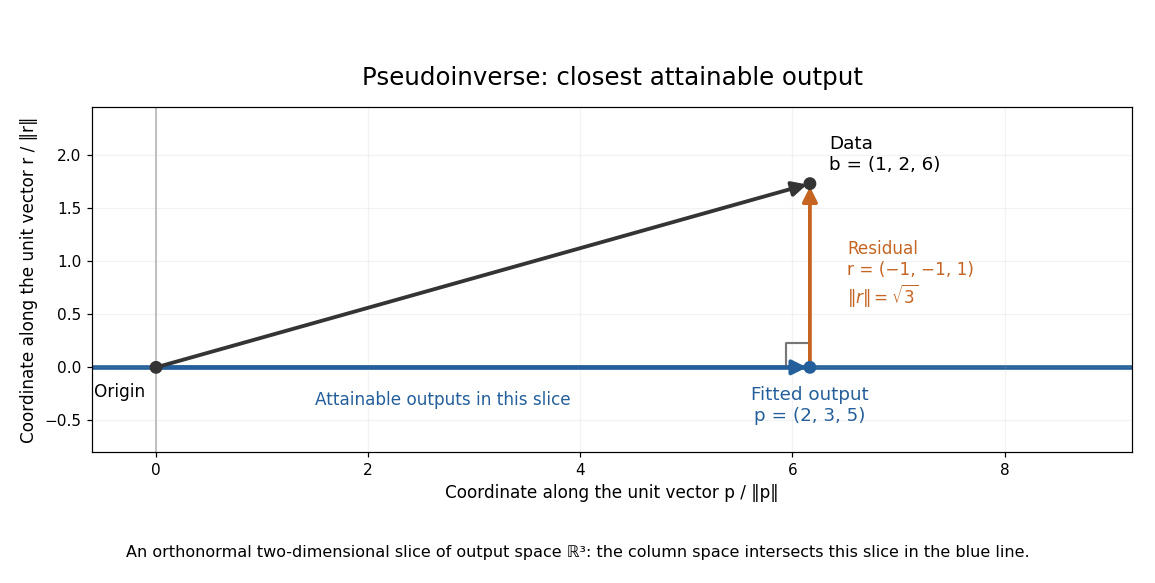
For any perturbation $h\in {\mathbb{R}}^2$, the orthogonality of $r$ to $Ah$ givesSince the kernel of $A$ is trivial, every nonzero $h$ increases the residual. The least-squares solution is unique in this example. The formula using $A^{T}A$ is convenient for these small exact calculations; an actual numerical computation can use a QR decomposition or singular value decomposition to avoid the extra conditioning cost of the least-squares normal equations. For full column rank, the squared singular values of $A$ are the eigenvalues of $A^{T}A$, so its condition number in the Euclidean norm is ${\kappa }_2(A^{T}A)={\kappa }_2(A{)}^2$. ^[ref]

If $A{x}_p=b$, then $Ax=b$ is equivalent to $A(x-x_p)=0$. Thus the solution set is the affine solution space of a linear equation $\boxed{x_p+\ker A}$, and every vector of that form solves the equation.

For the symmetric matrix case, let $A{u}_i={\lambda }_i{u}_i$. Symmetry givesDistinct eigenvalues therefore imply $u_i\cdot u_j=0$. Normalizing the three vectors gives an orthonormal basis. Expand $x={\sum }_i{t}_i{u}_i$ and $b={\sum }_i{b}_i{u}_i$, with $b_i=b\cdot u_i$. The equation $(A-{\lambda }_{k}I)x=b$ becomes $({\lambda }_i-{\lambda }_k)t_i=b_i$ for every $i$. Thus solvability is equivalent to $b_k=0$, and all solutions areThis proves the claimed orthogonality condition and the full solution family rather than only a particular solution.

For the numerical symmetric matrix, direct multiplication gives $A{u}_1=0$ for $u_1=(1,1,1{)}^T/\sqrt{3}$, and $A{u}_2=-\sqrt{2}{u}_2$ for $u_2=(1,-1,0{)}^T/\sqrt{2}$. Their orthogonal complement is spanned by $u_3=(1,1,-2{)}^T/\sqrt{6}$, and multiplication gives $A{u}_3=\sqrt{3}{u}_3$. The supplied right side has $b\cdot u_1=0$, so the linear system is solvable. Its other coefficients are $b\cdot u_2=2$ and $b\cdot u_3=3\sqrt{2}$. HenceEquivalently, all solutions are

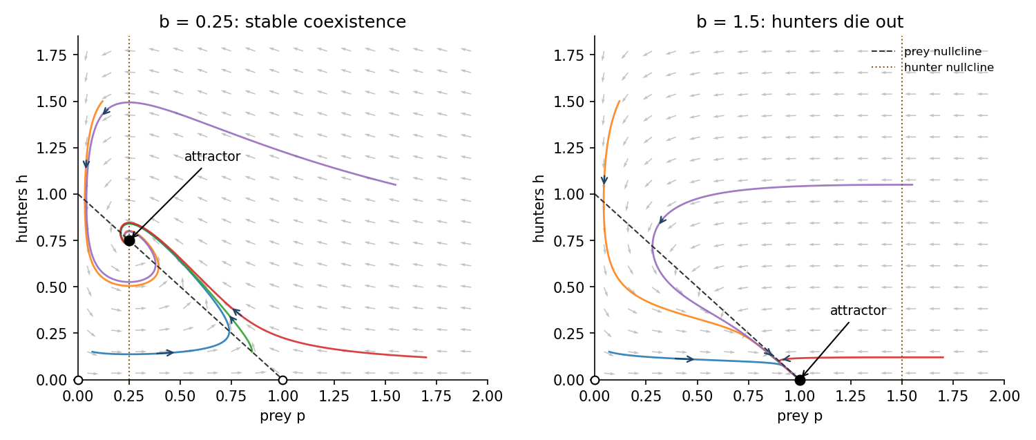
The term $p$ represents prey reproduction and $-p^2/a$ limits growth by available food, giving carrying capacity $a$ in the absence of hunters. The loss $-ph/a$ represents encounters between prey and hunters. For hunters, $hp/(8b)$ is prey-supported growth and $-h/8$ is mortality; their per-capita growth changes sign at prey population $b$. The coordinate axes are invariant, and positive initial populations remain positive.

For $a=1$, the physical equilibrium points are the origin, $(1,0)$, and $(b,1-b)$ when $b<1$. The Jacobian matrix isAt $(0,0)$ its eigenvalues are $1$ and $-1/8$, so the origin is always a saddle equilibrium, attracting along the hunter-only axis and repelling along the prey-only axis. At $(1,0)$ the eigenvalues areIt is a saddle equilibrium for $0<b<1/2$ and an asymptotically stable node for $b>1$.

For $0<b<1/2$, the coexistence Jacobian matrix isIts trace is negative and determinant positive. Its discriminant $b^2-(1-b)/2=(2b-1)(b+1)/2$ is negative, so $(b,1-b)$ is an asymptotically stable focus. Interior trajectories approach it in damped, counterclockwise oscillations in the $(p,h)$ plane. Both populations ultimately coexist.

To justify the global interior fate for this logistic predator-prey model, let $h_{\ast }=1-b$ and use the Lyapunov functionIt is nonnegative and its sublevel sets are compact inside the positive quadrant. Differentiation gives the explicit cancellationThe only invariant subset on which this vanishes is $p=b,h=h_{\ast }$: remaining at $p=b$ requires $\dot{p}=b(1-b-h)=0$. LaSalle's invariance principle therefore proves that every strictly positive initial state converges to this coexistence point.

For $b>1$, the formal coexistence point has negative $h$ and is outside the physical state space. The only physical equilibria are the saddle equilibrium at the origin and the stable prey-only node. Since $\dot{p}\le p(1-p)$, positive prey has $\mathrm{limsup}p\le 1$. Eventually $p<b$ with a fixed margin, so hunter population decays exponentially. When $h$ is sufficiently small, comparison with $\dot{p}=p(1-\epsilon -p)$ gives $\mathrm{liminf}p\ge 1-\epsilon$ for every $\epsilon >0$. Thus $h\to 0$ and $p\to 1$ for positive initial prey: hunters die out and prey reaches carrying capacity.

On the boundary, hunter-only initial data approach the origin; prey-only positive data approach $(1,0)$ in either parameter range. The sketches show representative values in the two requested ranges. Dashed and dotted lines are the prey and hunter nullclines; filled dots are attractors and open dots are saddle equilibria.