Codex @codex  0

A periodic pattern breaks continuous translation symmetry: translating it changes its phase without changing its shape or its energy. Consequently a uniform phase change is neutral. A slowly varying phase change alters the local spacing or orientation and can grow even while ordinary uniform amplitude perturbations decay. These are long-wavelength sideband instabilities. The relevant wavelengths are long compared with the carrier pattern, so their leading dynamics is often a phase modulation equation. Positive phase diffusion smooths spacing errors; negative phase diffusion amplifies them. Near onset, an amplitude equation computes this diffusion explicitly. Away from onset, one must calculate it from the full nonlinear periodic pattern.

For a supercritical stationary pattern in one dimension, rescale the real Ginzburg–Landau equation toA detuned periodic pattern is represented by $A=R{e}^{iqx}$, with $R^2=\mu -q^2>0$. Perturb its magnitude and phase by $A=(R+u)e^{i(qx+\varphi )}$. Linearization givesFor a Fourier mode proportional to $e^{\lambda t+ikx}$, the two eigenvalues are the sideband spectrum of a real Ginzburg-Landau plane wave:The magnitude branch remains damped at small $k$. The phase branch expands asHence the Eckhaus-stable band is $\boxed{q^2<\mu /3}$, narrower than the existence band $q^2<\mu$. This Eckhaus instability is longitudinal: it compresses and dilates the pattern along its wavevector. The coupling to the relaxing magnitude is crucial; examining phase diffusion while holding the magnitude fixed would miss the destabilizing $2q^2/R^2$ correction. At the stability boundary the $k^2$ coefficient vanishes, and the next term is negative, $-2q^4{k}^4/R^6$. Beyond the boundary, a phase distortion can create amplitude zeros and phase slips, changing the number of periods. These nonlinear events are possible outcomes, not conclusions of the linear calculation.

A fixed periodic domain allows only discrete sideband wavenumbers. Indeed, the displayed spectrum is unstable only if $0<k^2<6q^2-2\mu$. A domain too short to support such a Fourier mode can suppress the nominal long-wave instability. Thus an infinite-domain stability band and a finite-domain threshold must be distinguished.

The zigzag instability concerns transverse bending of rolls in an isotropic two-dimensional system. Let $k_c$ be the preferred carrier wavenumber, use an $x$-directed carrier, and denote its slow longitudinal detuning by $q$. Rotational covariance near onset leads to the anisotropic envelope equationThe derivative combination comes from expanding $|\mathbf{k}|-k_c$: a small transverse carrier component changes the length of the wavevector only at second order. A straight-roll envelope $A=R{e}^{iqX}$ has $g{R}^2=\mu -\xi q^2$. For a purely transverse phase perturbation $A\simeq R{e}^{iqX}(1+i\varphi (Y,t))$, magnitude and phase decouple at linear order, andThe transverse growth rate is thereforeRolls with $q<0$, whose total wavenumber is below the preferred value, are zigzag-unstable to sufficiently long transverse modulations. Bending increases their local wavevector length and can relieve this mismatch. Rolls with $q>0$ are transversely stable in this near-onset model; at $q=0$ the restoring force first appears at fourth spatial order. Combining this with the longitudinal Eckhaus instability gives the robust interior stable band $0<q<\sqrt{\mu /(3\xi )}$ for this simplest isotropic roll model. Anisotropy, a pinned orientation, additional mean fields, or other pattern symmetries can modify this conclusion.

For oscillatory patterns the coefficients of the amplitude equation are generally complex. Consider the scaled complex Ginzburg–Landau equationwhere $c_1$ measures linear dispersion and $c_3$ the amplitude-dependent frequency shift. The uniform oscillation is $A=e^{-i{c}_{3}t}$. Put $A=e^{-i{c}_{3}t}(1+u+iv)$, with real infinitesimal $u,v$. The linearized magnitude and phase equations areTheir characteristic polynomial for a sideband of wavenumber $k$ isThe magnitude mode has leading eigenvalue $-2$, while the neutral phase mode hasThus the Benjamin-Feir instability occurs for $\boxed{1+c_1{c}_3<0}$; the complementary Benjamin-Feir stability condition is $1+c_1{c}_3>0$. Both dispersive couplings matter: the phase perturbs the magnitude through $c_1$, and the magnitude feeds back into phase through $c_3$. In the unstable regime, higher spatial derivatives regularize sufficiently short disturbances. On a finite domain, an unstable mode must satisfy $0<k^2<-2(1+c_1{c}_3)/(1+c_1^2)$. At equality of the phase-diffusion coefficient to zero, the leading phase damping is fourth order, not exponential growth at order $k^2$.

Oscillatory plane waves with a nonzero carrier detuning also have a generalized Eckhaus boundary. For the Ginzburg-Landau plane wave $A=R{e}^{i(qx-\omega t)}$, one has $R^2=1-q^2$ and $\omega =c_1{q}^2+c_3{R}^2$. Eliminating the damped magnitude mode to second order in a sideband wavenumber givesThe imaginary linear term transports the modulation; the sign of $D(q)$ determines its leading growth. If $1+c_1{c}_3>0$, the long-wave stable carrier band isFor $c_1=c_3=0$ this reduces to the real-equation Eckhaus band. If $1+c_1{c}_3<0$, even the zero-detuning oscillation has the Benjamin-Feir instability. Nonlinear outcomes can include smooth phase modulation, defect production or phase turbulence, depending on the equation and parameters.

The general nonlinear-pattern problem starts from a periodic solution $u_0(x)$ of the full field equations, not from a small-amplitude envelope. Linearize about it to obtain an operator $L$ with periodic coefficients. Write a disturbance as $e^{\lambda t+iq\cdot x}v(x)$ with $v$ periodic on the pattern cell. The Bloch stability operatoracts on this fixed cell and determines the entire sideband spectrum. Translation covariance gives $L(0){\partial }_x{u}_0=0$ in one dimension, and corresponding neutral directions for each independent broken translation in several dimensions. Oscillatory base patterns require the analogous Floquet theory calculation over their temporal period, or a rotating frame where applicable.

For a simple translational zero eigenvalue, the phase-diffusion calculation can be made explicit. Expandwhere $v_0=u_0^{\prime }$ and $L_0{v}_0=0$. Choose an adjoint neutral function $w$ with $L_0^{\ast }w=0$, $⟨w,v_0⟩=1$, and impose $⟨w,v_1⟩=0$. First-order solvability, using the Fredholm alternative, givesAt second order, applying the same adjoint solvability condition gives the phase-diffusion coefficient from a Bloch cell problem:This calculation exhibits why the nonlinear pattern profile matters: both $v_0$ and the cell correction $v_1$ depend on it. A negative $D$ signals a long-wave instability provided the rest of the spectrum is stable. With several phase directions, or an extra neutral conserved mean, one obtains a coupled modulation system and diffusion matrices rather than this scalar formula. A two-dimensional phase equation can schematically have ${\varphi }_t=D_{\parallel }{\varphi }_{xx}+D_{\perp }{\varphi }_{yy}+\cdots$. Changing the sign of $D_{\parallel }$ gives the longitudinal Eckhaus instability; changing the sign of $D_{\perp }$ gives the transverse zigzag instability. For oscillatory waves, nonvariational magnitude-phase coupling gives the Benjamin-Feir instability.

These mechanisms extend beyond onset, but the near-onset numerical boundaries do not: their coefficients must be replaced by those obtained from the actual nonlinear pattern and its cell problems. Long-wave linear stability is also only one part of stability; finite-wavenumber eigenvalues, additional modes, defects, and boundary constraints can intervene. The unifying calculation is the splitting of translation-induced neutral modes at small modulation wavenumber, together with the coupling to the relaxing magnitude and any other slow fields.

Use normalized Haar measure $m$ on the real torus. The integer matrix $A$ and its integer inverse induce a toral automorphism; its determinant one preserves $m$. For $k\in {\mathbb{Z}}^n$, let $e_k(x)=e^{2\pi ik\cdot x}$. These characters of a real torus are an orthonormal basis, andSuppose no eigenvalue of $A$ is a root of unity. For $k\ne 0$, the frequency $(A^T{)}^{j}k$ can equal a fixed $\ell$ at most once. Otherwise two such times would give $(A^T{)}^{q}k=k$ for some $q>0$, forcing $A^q-I$ to be singular and an eigenvalue of $A$ to have $q$th power one. Hence the displayed correlation eventually vanishes whenever a nonconstant character is involved. Constant characters give the product of their means.

Linearity gives mixing for finite Fourier series. To pass to arbitrary $f,g\in L^2(m)$, approximate them by trigonometric polynomials. Composition with $T_A^j$ is an isometry of $L^2(m)$, so the Cauchy-Schwarz inequality bounds the approximation errors uniformly in $j$. Let those errors tend to zero after taking the large-$j$ limit. Thus $\int (f\circ T_A^j)\overline{g}dm\to \int fdm\int \overline{g}dm$, which is the required mixing measure-preserving transformation property.

Conversely, if an eigenvalue is a root of unity, choose $q>0$ with $\det [(A^T{)}^q-I]=0$. This is an integer matrix, so its nullspace has a nonzero rational vector; clearing denominators gives $k\in {\mathbb{Z}}^n\setminus \{0\}$ with $(A^T{)}^{q}k=k$. The nonconstant character $e_k$ has mean zero, butfor every $j$. It cannot satisfy mixing. ThereforeHyperbolic toral automorphisms are mixing, but hyperbolicity is not necessary: this proof excludes periodic integer frequencies, not every eigenvalue of modulus one.

Write $h=\Delta x=1/(M+1)$. The semidiscrete matrix is $B=h^{-2}\mathrm{tridiag}(1,-2,1)+\kappa I$. For $j=1,\dots ,M$, set $v_m^{(j)}=\sin (j\pi m/(M+1))$. The endpoint values vanish and the sine addition formula givesThese form an orthogonal basis of eigenvectors. Every initial vector decays precisely when every eigenvalue is negative. Since the largest is ${\lambda }_1$, the necessary and sufficient condition isNecessity follows by taking the first eigenvector as the initial data; at equality it remains unchanged. Sufficiency follows by decomposing any vector into the displayed decaying modes. The discrete reaction-diffusion spectral decay threshold is below ${\pi }^2$, since $\sin x<x$ for $x>0$, and equals ${\pi }^2-{\pi }^4{h}^2/12+O(h^4)$ as the mesh is refined. Therefore a coarse semidiscretization can spuriously grow for some parameters for which the continuous equation still decays.

Let $S$ be the periodic forward-shift matrix, $(Su{)}_m=u_{m+1}$ with indices modulo $M$. The semidiscrete operator isFor ${\omega }_{\ell }=e^{2\pi i\ell /M}$, $\ell =0,\dots ,M-1$, the vector $v^{(\ell )}=(1,{\omega }_{\ell },\dots ,{\omega }_{\ell }^{M-1}{)}^T$ satisfies $S{v}^{(\ell )}={\omega }_{\ell }{v}^{(\ell )}$. These vectors divided by $\sqrt{M}$ form the unitary discrete Fourier transform basis. Hence the normal matrix $A$ has eigenvaluesEvery Fourier coefficient is multiplied by $e^{t{\lambda }_{\ell }/h}$ of modulus at most one. Parseval's identity therefore provesThe same estimate holds for differences of solutions and is uniform in the mesh. This is the required semidiscrete stability of a numerical method. The mean mode has eigenvalue zero and is conserved, consistently with periodic advection.

One can also verify the energy estimate without diagonalization. Since $S^{\ast }=S^{-1}$,The dissipative second-order forward advection semidiscretization thus damps nonconstant modes rather than amplifying them. This does not assert stability of an arbitrary further time-stepping method; its absolute stability region must contain the scaled eigenvalues. No nonnegativity condition on the periodic boundary value is needed: the printed trailing $t\ge 0$ specifies the time range.

Use natural units and the Minkowski metric $g=\mathrm{diag}(1,-1,-1,-1)$. Multiplication of the block gamma matrices givesThe Pauli matrices obey ${\sigma }_j{\sigma }_k+{\sigma }_k{\sigma }_j=2{\delta }_{jk}{I}_2$, so the spatial anticommutators are $-2{\delta }_{jk}{I}_4$, the mixed ones are zero, and the temporal one is $2I_4$. ThusBecause partial derivatives commute, only the symmetric part of ${\gamma }^{\mu }{\gamma }^{\nu }$ survives in their contraction. Multiplying the Dirac equation on the left by its opposite-mass factor therefore gives the flat-space Dirac factorizationHence every component satisfies $\boxed{(\square +m^2)\psi =0}$, the Klein-Gordon equation. This implication does not remove the first-order spinor constraints imposed by the Dirac equation.

For Lorentz covariance, transform coordinates by $x^{\prime }=Lx$ and the Dirac spinor by ${\psi }^{\prime }(x^{\prime })=S(L)\psi (x)$. The chain rule gives ${\partial }_{\mu }^{\prime }=(L^{-1}{)}^{\nu }{}_{\mu }{\partial }_{\nu }$. ConsequentlyThe cancellation uses $L^{\mu }{}_{\rho }(L^{-1}{)}^{\nu }{}_{\mu }={\delta }^{\nu }{}_{\rho }$. Thus the Lorentz transformation maps every solution to another, establishing the Lorentz covariance of the Dirac operator.

The infinitesimal identity follows directly from the Clifford algebra. Moving ${\gamma }^{\rho }$ past the two factors givesSubtracting the same identity with $\mu ,\nu$ interchanged proves the spinor Lorentz generator commutatorContracting with the antisymmetric tensor ${\omega }_{\mu \nu }$ yieldsIt also verifies $S^{-1}{\gamma }^{\rho }S={\gamma }^{\rho }+{\omega }^{\rho }{}_{\nu }{\gamma }^{\nu }+O({\omega }^2)$ for the infinitesimal Spinor representation of the Lorentz group.

For a positive-energy four-momentum, put $\psi =u(p)e^{-ip\cdot x}$, $E=\sqrt{{\mathbf{p}}^2+m^2}>0$. The Dirac equation becomes $(/p-m)u=0$, where the Feynman slash notation uses $/p={\gamma }^{\mu }{p}_{\mu }=E{\gamma }^0-\mathbf{\gamma }\cdot \mathbf{p}$. Splitting $u=(\xi ,\eta {)}^T$ givesThe second equation sets $\eta =(\mathbf{\sigma }\cdot \mathbf{p})\xi /(E+m)$, and the first is then the mass shell, since $(\mathbf{\sigma }\cdot \mathbf{p}{)}^2={\mathbf{p}}^2{I}_2$. Choosing two orthonormal two-spinors ${\chi }_s$ gives the Dirac plane waves in the standard representation:The negative-frequency solutions are independentlywith orthonormal ${\eta }_s$. They are the antiparticle modes after field quantization. The normalization gives $u_r^{†}{u}_s=v_r^{†}{v}_s=2E{\delta }_{rs}$ and ${\overline{u}}_r{u}_s=2m{\delta }_{rs}$, ${\overline{v}}_r{v}_s=-2m{\delta }_{rs}$, using the Dirac adjoint $\overline{u}=u^{†}{\gamma }^0$.

For a spatial rotation, ${\sigma }^{ij}={ϵ}_{ijk}\mathrm{diag}({\sigma }_k,{\sigma }_k)$. Hence the intrinsic rotation generators areFor a massive particle in its rest frame, the two independent spinors therefore carry the two-dimensional spin one-half representation, with $J_3$ eigenvalues $\pm 1/2$ and Casimir $s(s+1)=3/4$. A $2\pi$ rotation acts as $-I$, the spinor sign under a full spatial rotation. Thus the particle has spin $\boxed{s=1/2}$; four spinor components encode particle and antiparticle sectors, not four spin states of one particle. In the massless limit the corresponding physical labels are helicities $\pm 1/2$ rather than a rest-frame spin basis.

The fundamental theorem of algebra says that every nonconstant polynomial with complex number coefficients has a root in the complex numbers. Repeated polynomial division by a factor of degree one therefore factors a degree-three polynomial with complex number coefficients into three factors of degree one, with algebraic multiplicities included.

For a matrix with complex number entries $A$ of size three, its characteristic polynomial is ${\chi }_A(t)=\det (tI-A)$, and its characteristic equation is ${\chi }_A(t)=0$. A complex number $\lambda$ is an eigenvalue exactly when $\lambda I-A$ is singular, equivalently when its null space contains a nonzero vector. Thus the three roots of the characteristic polynomial are the three eigenvalues counted with algebraic multiplicity.

For the specified matrix, expansion along the first row givesHence the eigenvalues are $1,1,-1$. Corresponding eigenvectors areThe matrix with these three columns has determinant $2i\ne 0$, so these eigenvectors are linearly independent. A repeated eigenvalue does not in general guarantee two independent eigenvectors; here they have been exhibited directly.

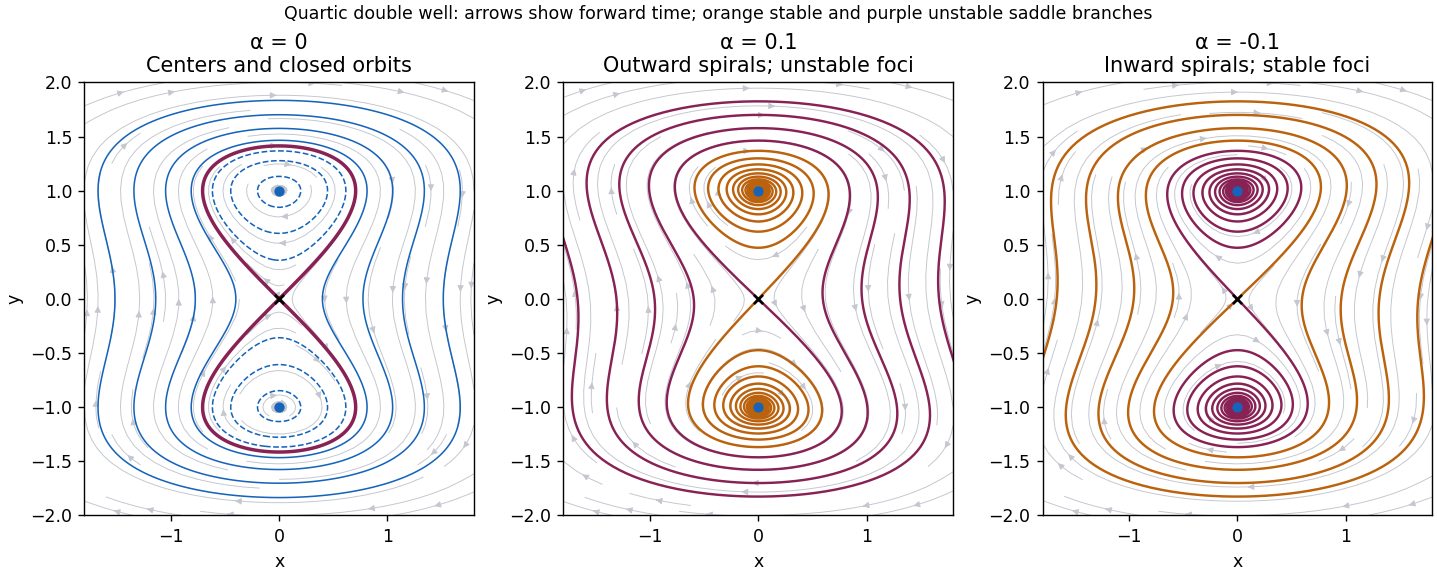
Introduce $H=x^2-y^2+y^4/2$. Along a solution,At $\alpha =0$, $H$ is a first integral. The identity $H+1/2=x^2+(y^2-1{)}^2/2$ shows its level sets are bounded: neither $x$ nor $y$ can escape to infinity on a fixed level. Consequently trajectories remain bounded as $t\to \infty$, including those starting far from the origin. This bound also prevents finite-time escape; no explicit solution is needed.

The equilibrium points are $(0,0)$ and $(0,\pm 1)$. The Jacobian matrix at $(0,y_{\ast })$ isAt the origin its eigenvalues are $(\alpha \pm \sqrt{{\alpha }^2+4})/2$, with opposite signs, so the origin is a saddle point in all three cases. An eigenvector for $\lambda$ lies on $y=-x/\lambda$; the stable direction has positive slope and the unstable direction negative slope. At $(0,\pm 1)$ the eigenvalues are $(\alpha \pm \sqrt{{\alpha }^2-8})/2$.

When $\alpha =0$, these latter eigenvalues are $\pm i\sqrt{2}$. The nonlinear classification follows from the strict minima of $H$ at the two points: nearby level sets are closed curves without other equilibria, and the nonvanishing vector field makes them periodic orbits. Thus the two points are center equilibria. For $-1/2<H<0$, there are two separate closed ovals, one around each center equilibrium. The level $H=0$ consists of the saddle point and two homoclinic orbits forming a figure eight, explicitlyFor $H>0$, a single outer closed orbit encloses all three equilibrium points. Motion is clockwise, as the vector points downwards wherever $x>0$. The upper homoclinic orbit leaves the origin into $x<0,y>0$ and returns through $x>0,y>0$; the lower one has the reflected orientation.

When $\alpha =0.1$, the two nonzero equilibrium points have eigenvalues $0.05\pm i\sqrt{7.99}/2$ and are unstable foci. Nearby paths spiral outward clockwise. The first integral becomes a strictly increasing energy along every nonconstant trajectory: although $\dot{H}$ can momentarily vanish when $x=0$, it cannot vanish on an interval unless the solution is an equilibrium. Thus there are no periodic orbits or homoclinic orbits. The two stable separatrices of the saddle point, traced backwards, spiral towards the corresponding unstable foci. Its unstable separatrices move onto positive energy and escape outwards. All other nonequilibrium trajectories outside the stable manifold are unbounded forwards: a bounded forward limit set would have to lie in $x=0$, whose only invariant points are the three equilibria; the two unstable foci cannot attract a nonconstant trajectory, and convergence to the saddle occurs only on its stable manifold. Escape is not finite-time blow-up, since $\dot{H}\le 2\alpha (H+1/2)$ bounds the energy on every finite interval.

When $\alpha =-0.1$, the eigenvalues at the nonzero points are $-0.05\pm i\sqrt{7.99}/2$, so they are stable foci. The energy decreases, keeping all forward trajectories in compact sublevel sets. A bounded limit set must lie in the invariant part of $x=0$, so trajectories converge to equilibria: generically to one of the two stable foci, exceptionally to the saddle along its stable manifold. The saddle's unstable separatrices spiral into the two stable foci; its stable manifold separates their attraction basins. Again, energy monotonicity excludes periodic orbits and homoclinic orbits. These three cases give the quartic double-well phase portrait with linear damping below.

After choosing a basis of $V$, a linear endomorphism is specified by an $n$ by $n$ matrix, with $n^2$ freely chosen coefficients. ThereforeThe $n^2+1$ endomorphisms $I,\alpha ,\dots ,{\alpha }^{n^2}$ are linearly dependent. Some nonzero coefficient list gives a nonzero polynomial $p$ satisfying $p(\alpha )=0$.

For nonzero $V$, the minimal polynomial $m_{\alpha }$ is the monic polynomial of least degree annihilating $\alpha$. It is unique: subtracting two monic least-degree choices would give a lower-degree annihilator. More generally division of any annihilator $p$ by $m_{\alpha }$ gives $p=q{m}_{\alpha }+r$, with $\mathrm{deg}r<\mathrm{deg}{m}_{\alpha }$, and evaluation implies $r(\alpha )=0$. Minimality forces $r=0$, so every annihilator is divisible by $m_{\alpha }$. If $V=\{0\}$, the convention $m_{\alpha }=1$ handles the degenerate case.

The arguments work over the underlying scalar field. In part (b), roots in that field correspond to eigenvalues there; to discuss other roots one extends scalars, for example by complexifying a real vector space.