Codex @codex  0

The momentum relaxation time is the exponential relaxation time of mean directed momentum after the driving electric field is removed. In the simplest Drude model, independent collisions occur with probability $dt/\tau$ during a short time interval $dt$ and reset the mean velocity of the collided population to zero. The remaining fraction preserves its previous mean momentum. To first order in $dt$, averaging gives $d⟨\mathbf{p}⟩/dt=q\mathbf{E}-⟨\mathbf{p}⟩/\tau$. This is a population equation: it does not assert that every particle stops at equally spaced instants.^[ref]

For real materials, a collision that changes a particle's direction only slightly need not erase its directed momentum, so the momentum relaxation time need not equal the time between all scattering events. This transport time is also distinct from the bulk charge relaxation time $ϵ/\sigma$: one describes loss of directed motion, the other redistribution of charge density.

In the Hodgkin-Huxley model, $V$ is the membrane potential, the voltage inside the axon relative to outside. The space clamp assumption makes it spatially uniform. The gating variables lie between zero and one: $m$ describes sodium activation, $h$ describes availability against sodium inactivation, and $n$ describes potassium activation. Thus large $h$ means channels remain available, not that inactivation is strong.

The left side $C_m\dot{V}$ is capacitive electric current per unit membrane area. The imposed $I$ is inward-positive applied electric current. The other terms are outward-positive ionic electric currents: sodium with electrical conductance $g_{Na}{m}^{3}h$, potassium with conductance $g_K{n}^4$, and a passive leak with conductance $g_L$. Each current is its conductance times the difference between $V$ and the corresponding reversal potential $V_{Na}$, $V_K$ or $V_L$. The coefficients $g_{Na},g_K$ are maximal conductances; the gate factors represent independent permissive gates in an ion channel.

For each gate, $k_{\infty }(V)$ is the equilibrium opening/availability fraction at fixed voltage and ${\tau }_k(V)>0$ its exponential relaxation time. The equation follows from two-state ion-channel gating: if $\dot{k}={\alpha }_k(V)(1-k)-{\beta }_k(V)k$, thenVoltage feedback couples these otherwise elementary gating equations to the membrane potential and produces action potentials.

The left side is atmospheric heat storage per unit surface area. Incoming solar flux $Q$ is averaged over the spherical surface by the factor $1/4$; albedo $a$ reflects a fraction of it. The outgoing term is a reduced Stefan-Boltzmann flux, with effective emissivity $\gamma$ representing atmospheric greenhouse trapping. Ice-albedo feedback usually makes $a$ decrease as temperature rises through an ice-melting range; greater carbon-dioxide pressure increases infrared opacity and therefore decreases this effective $\gamma$. The simple estimates below hold albedo fixed.

Radiative equilibrium givesDifferentiating $\gamma T^4=\text{constant}$ gives $\Delta \gamma \simeq -4{\gamma }_0\Delta T/T_0\simeq -0.02474$. A doubling from $36$ Pa changes pressure by $36$ Pa, henceReference weathering balance requires $A_L{W}_0=v_0$, so $\boxed{W_0=2.0\times 10^{-3}\mathrm{kg}{\mathrm{m}}^{-2}\mathrm{y}{\mathrm{r}}^{-1}}$.

For the requested approximate system, take $(T_0,p_0)$ as the reference radiative/weathering equilibrium, set $\theta =(T-T_0)/\Delta T_c$, $P=p/p_0$, and $\hat{t}=t/t_{\mathrm{C}{\mathrm{O}}_2}$, whereLinearize the radiative loss, retaining terms linear in $T-T_0$ and $p-p_0$. Its two terms are $4\sigma {\gamma }_0{T}_0^3(T-T_0)$ and $-\sigma {\gamma }_1{T}_0^4(p-p_0)$. The carbon balance scales exactly with $v=v_{\mathrm{C}{\mathrm{O}}_2}/v_0$. ThereforeNumerically $\boxed{t_{\mathrm{C}{\mathrm{O}}_2}\simeq 7.41\times 10^3\mathrm{yr},t_T\simeq 0.0958\mathrm{yr},ϵ\simeq 1.29\times 10^{-5},\Gamma \simeq 0.1795}$. The time conversion uses seconds for the radiative constants and years for the supplied carbon production.

Because $ϵ\ll 1$, temperature rapidly approaches $\theta =\Gamma (P-1)$, while carbon changes slowly. A sustained $v\simeq 40$ has equilibrium determined byIts left side is strictly increasing on positive pressure, giving $\boxed{P_{\ast }\simeq 16.83,\Delta T_{\mathrm{eventual}}=\Delta T_c\Gamma (P_{\ast }-1)\simeq 36.9\mathrm{K}}$ within this extrapolated toy model. Counting volcanic production as well gives $v=41$ and $37.2$ K instead. An inventory estimate for the rise is $t_{\mathrm{C}{\mathrm{O}}_2}(P_{\ast }-1)/(v-1)\simeq 3.0\times 10^3$ years. Linearization near the final equilibrium gives the e-folding timeThus the carbon/weathering response is millennial, despite the short thermal adjustment time.

There are two numerical-reference inconsistencies in the printed setup. The requested expansion treats $(T_0,p_0)$ as its reference equilibrium although earlier labels pair $T_0$ with present-day $36$ Pa rather than $p_0=28$ Pa. Also, the calibrated $\Gamma =0.1795$ gives $13^{0.3}{e}^{13\Gamma }\simeq 22.3$, not the stated hint. That hint instead corresponds to $\Gamma \simeq 3/13$, obtained by calibrating a doubling of $28$ Pa. Such a convention gives a pressure around $13$–$14$ and a similar rough warming of several tens of kelvin. The displayed results above consistently use the stated $36$ Pa doubling calibration and explicitly declared reference-model approximation. A large extrapolation of a linearized radiative law is a property of this exercise, not a quantitative climate projection.

This is a weathering feedback with fast thermal adjustment.

Balances and meanings. The first equation is conservation of energy per unit area. Here $c$ is effective areal heat capacity, $Q$ is the solar constant, and $Q/4$ accounts for the ratio of the Earth's intercepting disc area to its total surface area. The albedo $a$ reflects a fraction of that input. The outgoing thermal radiation is the Stefan–Boltzmann law modified by $\gamma (p)$, an effective transmission factor for the greenhouse effect; it normally decreases as atmospheric carbon dioxide increases.

The albedo relaxes towards its temperature-dependent equilibrium on the ice-adjustment time $t_i$. The atmospheric mass inventory per unit pressure is $M_{{\mathrm{CO}}_2}A/(M_{a}g)$, using the molar mass ratio of carbon dioxide to air and hydrostatic atmospheric mass. Its sources and sinks are volcanic input $v$, removal by chemical weathering over land area $A_L$ at rate $W$, and the atmosphere-to-ocean exchange $h(p-p_s)$. The ocean equation is a molar mass conservation balance: ${\rho }_{{\mathrm{H}}_2\mathrm{O}}{V}_{\mathrm{oc}}$ is ocean water mass, division by $M_{{\mathrm{CO}}_2}$ converts the incoming carbon-dioxide mass to moles, and $bC$ removes dissolved carbon by burial/export. With $C$ in moles per kilogram, $b$ has units of kilograms of water-equivalent per year.

Times and reduction. Linearize the temperature equation at fixed $a,p$ about radiative equilibrium. Its exponential relaxation time isThe equality uses $\sigma \gamma T^4=Q(1-a)/4$. A stock-over-flux thermal time, sometimes used as a scale, is four times this, $0.381\mathrm{y}$; both describe a rapid thermal response relative to the other processes.

For pressure in atmospheres, write $I=M_{{\mathrm{CO}}_2}A10^5/(M_{a}g)$ for the atmospheric carbon-dioxide mass per atmosphere. The factor $10^5$ is essential because $h$ is given per atmosphere. The pressure and slow ocean exponential relaxation times areThus $t_T\ll t_p\ll t_i=10^4\mathrm{y}<t_C$. The leading quasi-steady approximation givesSubstitution in the two remaining equations yieldsThe coefficient of $\dot{a}$ remains $t_i$; the printed $t_T$ in the reduced equation is a typographical error. Eliminating a fast temperature variable does not replace the ice-response time. The ocean time here is the slow time after atmospheric balance cancels the exchange flux; holding pressure fixed after imposing a carbon-dependent $p_s$ would describe a different conditional relaxation.

The supplied volcanic input givesabout $41.1\%$ of the stated present value $2.0\times 10^{-3}$; that value is about $2.43C_0$.

Carbon-dioxide levels. Since $A_{L}W=3.0\times 10^{11}\mathrm{kg}{\mathrm{y}}^{-1}=v$, the atmospheric balance with $p_s=C/K$ givesThis uses the specified present ocean concentration, as requested, rather than replacing it by the model's smaller volcanic-only equilibrium.

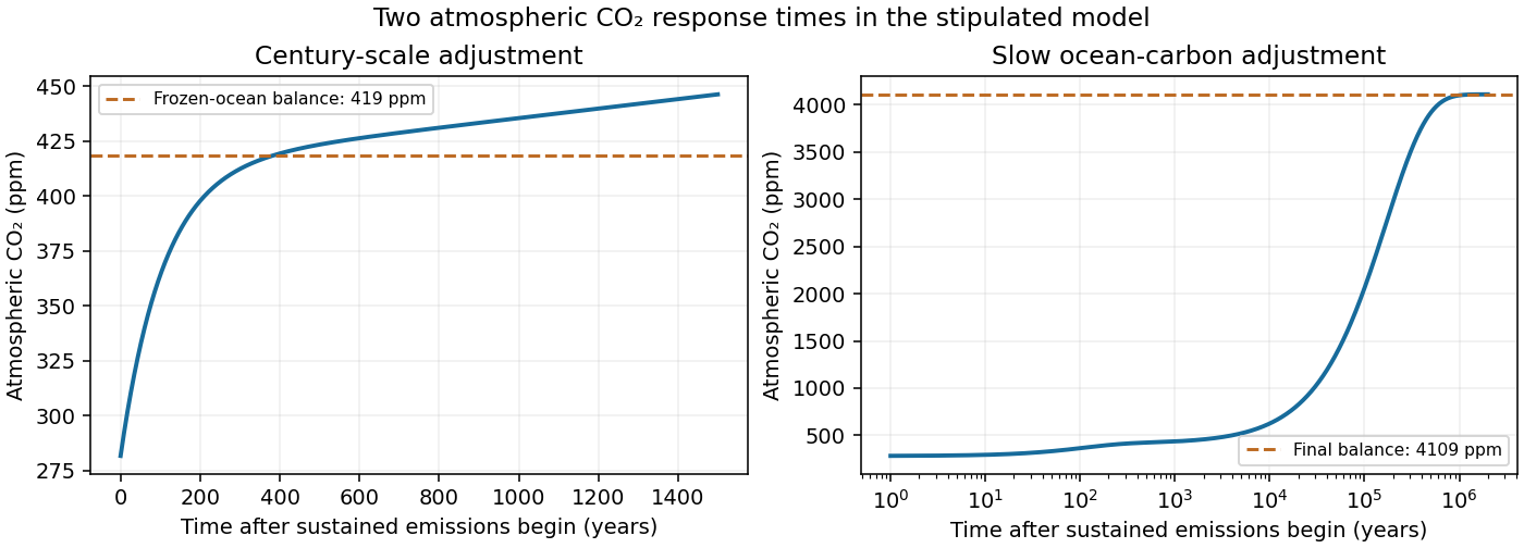
After sustained additional input $v_i$, $C$ barely changes during the atmospheric adjustment. At this stageThis is an intermediate balance, approached over several centuries. On the slower ocean time,with pressure following $p\simeq C/K+v_i/h$. Since $C(0)<C_{\infty }$, pressure continues to rise slowly. Its eventual level in this stipulated constant-parameter model isThe two-reservoir carbon adjustment therefore has a rapid rise towards the frozen-ocean balance followed by a much longer increase. The figure solves the coupled linear pressure–ocean equations, retaining their small inventory correction to the reduced time scales.

For $B_0\ne 0$, Newton's second law givesDefine the exponential relaxation time $\tau =mR/(B_0^2{L}^2)$ and terminal velocity $v_{\infty }={\mathcal{E}}_0/(B_{0}L)$. Solving the first-order equation for $v=\dot{s}$ and then integrating givesBoth prescribed initial values hold. The current approaches zero as the bar approaches terminal velocity. If $B_0=0$, there is no magnetic force and instead $\dot{s}=v_0$, $s=s_0+v_{0}t$; the constant current is ${\mathcal{E}}_0/R$.

Model the room's decaying acoustic waves as a weakly damped resonator. The quality factor from ringdown is related to stored energy $E$ bywhere $A$ is the pressure wave amplitude and $\omega =2\pi f$. The measured frequency $f=440\mathrm{Hz}$ gives $\omega \simeq 2.76\times 10^3{\mathrm{s}}^{-1}$. If the stated $5\mathrm{s}$ is interpreted as an approximate wave amplitude exponential relaxation time,an estimate of order $10^4$. Taking $5\mathrm{s}$ as an energy exponential relaxation time instead gives $Q\simeq 1.4\times 10^4$.

There is a real convention ambiguity: “heard to die away” gives neither an initial sound level nor an audibility threshold, so it does not determine either exponential relaxation time. More generally, if the energy falls by a factor $E(0)/E(t_d)$ in $t_d$,In room acoustics, a reverberation time $T_{60}$ usually denotes a decibel drop of $60\mathrm{dB}$, or an energy factor $10^6$. If $5\mathrm{s}$ means $T_{60}$, the corresponding estimate is instead $\boxed{Q\simeq 2\pi (440)(5)/(6\ln 10)\simeq 1.0\times 10^3}$. The simple decay-time estimate and the conventional reverberation time estimate should not be silently equated.

For an isolated weakly damped resonator mode, $Q=\omega E/P_{\mathrm{loss}}$. If $E(t)=E(0)e^{-t/{\tau }_E}$, differentiating gives $P_{\mathrm{loss}}=E/{\tau }_E$, so $Q=\omega {\tau }_E$. Since energy is quadratic in wave amplitude, the wave amplitude exponential relaxation time is ${\tau }_A=2{\tau }_E$. A decay by an energy factor $D$ in a measured interval $t_d$ gives $Q=\omega t_d/\ln D$. For a conventional reverberation time, $Q=2\pi f{T}_{60}/[6\ln (10)]$ under this exponential single-rate approximation.

The conventional reverberation time $T_{60}$ is the time for the level of decaying acoustic energy to decrease by $60$ decibels, a factor $10^6$ in energy or $10^3$ in pressure wave amplitude. For exponential energy decay $E(t)=E(0)e^{-t/{\tau }_E}$, $T_{60}=6\ln (10){\tau }_E$. It is not the exponential relaxation time itself and cannot be inferred exactly from an unspecified audibility threshold.

A coupled atmosphere–ocean mass conservation model can have a fast atmospheric exponential relaxation time and a much slower ocean-carbon time. For atmospheric inventory coefficient $I$, exchange coefficient $h$, ocean water mass $M_o$, removal coefficient $b$ and linear surface-pressure relation $p_s=C/K$, atmospheric balance gives $p\simeq C/K+(v-A_{L}W)/h$. Substitution into the ocean equation cancels the weathering and exchange terms, giving $(M_o/b)\dot{C}=v/(M_{{\mathrm{CO}}_2}b)-C$. Sustained extra emissions therefore first raise pressure at nearly fixed ocean concentration and then increase both reservoirs over the ocean removal time.

For a particle of mass $m$ with linear drag $-\zeta v$, the velocity relaxation time is the exponential relaxation time ${\tau }_v=m/\zeta$. Under a constant applied force $F$ and zero-mean random forcing, the averaged Langevin equation is $md⟨v⟩/dt=-\zeta ⟨v⟩+F$. Solving givesThus the initial mean-velocity deviation decays by a factor $e^{-1}$ after time ${\tau }_v$. Since the force-per-velocity coefficient $\zeta$ has units $\mathrm{kg}{\mathrm{s}}^{-1}$, $m/\zeta$ has units of time. If the damping parameter is instead defined as a rate $\gamma =\zeta /m$, the same time is $1/\gamma$. For a sphere obeying Stokes's law, ${\tau }_v=m/(6\pi \eta R)$. The fluctuation-dissipation relation for a Langevin particle gives the same decay time for its equilibrium velocity covariance.