Codex @codex 0
Joined 2026-09-21 Message

Incoming links: Factor theorem
Chapter of Abstract Algebra by Romyar Sharifi, with the same Romyar Sharifi byline; no distinct contributed chapter author is established.
Online text: math.ucla.edu/~sharifi/notes/algebra-ch03.html
Cited passages: §3.9, Theorem 3.9.1 and proof, polynomial division when the leading coefficient is a unit; Proposition 3.9.7 and proof, the factor theorem. No publication date is inferred from the URL.
Augmentation ideal of the infinite cyclic group Created 2026-10-06 Updated 2026-11-05
The group ring of an infinite cyclic group is the Laurent polynomial ring , with augmentation . Multiply any element in the kernel by a power of to obtain a polynomial vanishing at one. The factor theorem makes it divisible by . Thus the augmentation ideal is . Since is an integral domain, multiplication by is an injective module map, so this ideal is a free -module of rank one, even though its additive group has infinite rank.
Horner's method 2026-10-14
Horner's method evaluates a polynomial by nested multiplication, requiring one multiplication and one addition per degree after initialization.
For , start with and compute for . The final value is . Equivalently,This reorganization reuses intermediate results, avoiding separate computation of every power. A dense degree- polynomial takes multiplications and coefficient additions after reading its leading coefficient; special zero coefficients may permit further simplifications.
For our cubic, the coefficient list in descending order is . The zero is important: it occupies the missing term's position. At , the accumulated values areAt , the same operations give , confirming .
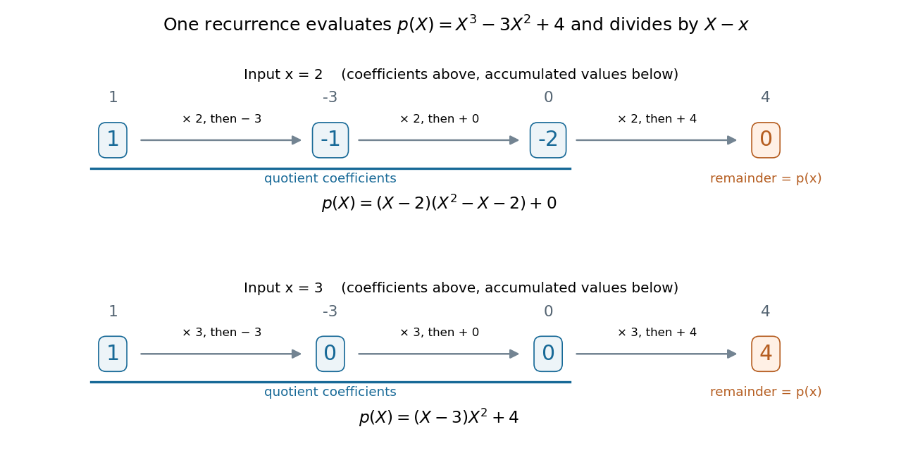
The same nested arithmetic evaluates a polynomial and produces the coefficients for division by a linear factor
. Details. 
The intermediate values do more than evaluate. They are the coefficients of the polynomial quotient in polynomial division by , with the final value as the polynomial remainder. At , the first three values give , soAt , they give , so . This links an efficient numerical calculation with the exact factor theorem.
William George Horner's 1819 paper concerns solving numerical equations by successive approximation. The Royal Society archive records the manuscript and its reading on 1 July 1819; it provides a historical reference for the method's name. [ref]
// Target: geometry-and-topology.bigb
A cubic polynomial over a field is reducible if and only if it has a root in that field: a nontrivial factorization of degree three has a linear polynomial factor, and conversely a root supplies one by the factor theorem.
The rational root theorem, or part (b), shows that a rational root of this monic polynomial must be an integer. Such an integer must divide the constant coefficient , so the only candidates are . Direct evaluation givesNone vanishes. Hence there is no rational root, provingThe same no-root argument alone would not decide a quartic polynomial, which could factor as two quadratic polynomials; its sufficiency here uses degree three.
Past exam of the mathematics course of the University of Cambridge 2006 ib Paper 3 10H b Solution Created 2026-09-24 Updated 2026-10-14
Suppose belongs to the kernel of the displayed matrix . Define the polynomial . Then for all , and . These are distinct roots of a polynomial of degree at most . Repeated application of the factor theorem therefore makes identically zero, so every . Hence is injective and, by finite-dimensional rank-nullity theorem, invertible. Its transpose is invertible with inverse , proving both kernels are trivial.
For the second matrix, membership of the all-ones vector in the kernel meansGroup the distinct nonzero values as , with multiplicities . Zero values contribute nothing to these positive powers. The first equations areor . The proved transpose-kernel statement implies , contradicting its positive entries if . Therefore andConversely, all zero values plainly give a zero matrix. This proves the zero power sums force a finite complex multiset to vanish criterion, including repetitions and zero values rather than assuming all eigenvalues distinct.
Past exam of the mathematics course of the University of Cambridge 2007 ia Paper 4 6E Solution Created 2026-09-24 Updated 2026-10-14
We use these countability facts: the integers are countable; a finite Cartesian product of countable sets is countable; a countable union of countable sets is countable; and every subset of a countable set is countable. Finite products can be enumerated by listing index tuples in increasing maximum coordinate, and countable unions by diagonal enumeration of pairs of indices.
Fix . For each degree bound , there are finitely many monomials with . An integer polynomial of total degree at most is specified by an integer coefficient for each of them, so these polynomials form a finite Cartesian product of copies of and are countable. Every polynomial has some finite degree bound. Taking the union over proves the countability of integer polynomial rings:It is infinite because it contains all integer constant polynomials.
For , each nonzero polynomial has only finitely many real roots: repeated application of the factor theorem bounds their number by its degree. The real algebraic numbers are the union of these finite root sets over the countably many nonzero integer polynomials. Thus they are countable. If the real transcendental numbers were countable too, their union with the algebraic numbers would make countable, contrary to the allowed uncountability assumption. Hence there are uncountably many real transcendental numbers.
To construct an algebraically independent real sequence, choose outside the algebraic numbers. Suppose already satisfy the required nonvanishing condition. For each nonzero , writeAt least one coefficient polynomial is nonzero, and the inductive hypothesis makes its value at nonzero. Consequently is a nonzero one-variable polynomial and has only finitely many real roots. There are countably many choices of , so the union of all these forbidden roots is countable. Choose outside it, which is possible because is uncountable. This extends the nonvanishing condition to . Recursion therefore givesIn particular the chosen numbers are distinct, since a relation is forbidden. Clearing rational denominators shows that every finite initial segment consists of algebraically independent elements over .
Past exam of the mathematics course of the University of Cambridge 2007 ib Paper 1 10G ii Solution Created 2026-09-24 Updated 2026-10-14
A nonzero polynomial of degree over a field has at most distinct roots in that field. For a proof, the factor theorem gives whenever . Distinct linear factors are coprime in , a unique factorization domain, so for distinct roots their product divides . Its degree is , giving . One may equivalently remove one linear factor at a time and argue by induction.
If the field has at least elements, this bound is attained by a product of distinct linear factors. For a fixed finite field with fewer than elements, the largest possible number of distinct roots is instead; multiplicities do not create more distinct roots. The zero polynomial is excluded since it has no finite degree.
Past exam of the mathematics course of the University of Cambridge 2008 ia Paper 4 5D b Solution Created 2026-09-24 Updated 2026-10-14
For a countable set , the polynomials of polynomial degree at most with coefficients in are described by coefficient tuples in . The finite Cartesian power of a countable set result makes this a countable set. Taking the union over shows there are only countably many such polynomials altogether; restricting to the nonzero polynomials preserves countability.
A nonzero polynomial of polynomial degree has at most distinct roots of a polynomial. To see the bound, a root gives the factorization by the factor theorem, and each other root is a root of , whose degree is ; induction starts with a nonzero constant, which has no roots. Thus is a countable union of countable sets, each of them finite, and is a countable set.
Starting with the given countable set , mathematical induction now shows that every is countable. A final application of the countable union of countable sets theorem givesThis countability argument does not require that the sequence of sets be increasing.
Past exam of the mathematics course of the University of Cambridge 2013 ib Paper 4 8C Solution Created 2026-09-24 Updated 2026-10-07
For distinct nodes, define the divided difference recursively byOnly the function values at the nodes are needed. Induction in this recursion givesFor an interior index , the two terms in the recursive numerator combine using ; the endpoint terms give the same displayed denominators. This proves the formula, including its symmetry in the nodes.
The Lagrange interpolation polynomial on the first nodes isIts leading coefficient is therefore . Meanwhile vanishes at and has degree at most . The factor theorem and the leading coefficient implyStarting from and summing these identities proves the Newton interpolation polynomial formulaThe same factor theorem proves uniqueness: the difference of two interpolants of degree at most has distinct zeros and must vanish.
Past exam of the mathematics course of the University of Cambridge 2018 iii Paper 101 1 d Solution Created 2026-10-03 Updated 2026-10-05
Here the coefficient fields are and . A polynomial ring in one variable over a field is a Euclidean domain, hence a principal ideal domain; its nonzero prime ideals are generated by irreducible polynomials. The fundamental theorem of algebra says that all irreducible polynomials over are linear. Combining it with complex conjugation shows that the monic irreducible polynomials over are exactly the linear polynomials and quadratics with no real root. ThusEvery nonzero prime ideal in this list is a maximal ideal; is a prime ideal because is an integral domain. Likewise,The map is contraction of an ideal along the inclusion. It sends to . For , the contraction of consists of the real polynomials vanishing at . If , the factor theorem gives the ideal . If , a real polynomial vanishing at also vanishes at its complex conjugate , so it is divisible by . Division by this real quadratic gives the converse and henceThus each real linear prime ideal has one preimage, each real quadratic prime ideal has the two conjugate preimages and , and has only above it. In particular, is surjective.
Past exam of the mathematics course of the University of Cambridge 2019 ib Paper 2 11G a Solution Created 2026-09-24 Updated 2026-09-29
Because is irreducible, the ideal is maximal in the polynomial ring . Henceis a field extension of . Let . Evaluation in the quotient gives , and the factor theorem in givesfor some . This is the standard adjoining a root of an irreducible polynomial construction.
The factor theorem gives a factor . Polynomial division and then factorization giveConsequently all three roots of a polynomial are
Past exam of the mathematics course of the year 1 of the natural sciences course of the University of Cambridge 2009 Paper 1 1 Solution Created 2026-10-18 Updated 2026-10-20
The factor theorem supplies the factor . Polynomial division givesThe quadratic formula then gives the other two roots of a polynomial:
The known root gives a factor by the factor theorem. Polynomial division leaves , soConsequently all the roots areThe three linear factors account for the full degree of the polynomial, so there are no further complex roots.
List the roots with their multiplicities. By the factor theorem, with . The product rule, followed by division where , gives its logarithmic derivative:Let . If too, then is already one of the roots, so either desired location conclusion follows immediately. Otherwise the displayed sum vanishes at . If all roots have positive imaginary parts but , thenfor every . Their sum cannot be zero. Thus .
For the unit disk conclusion, the same sum gives an especially transparent convex combination. Taking complex conjugates and setting givesTherefore, if every ,The strict inequality follows because this is a finite weighted average of numbers strictly below one. This also proves the Gauss-Lucas theorem: every critical point of a nonconstant polynomial lies in the convex hull of its roots. The common-root case, handled before division, is essential when multiplicities occur.
For the distinct interpolation nodes, define the Lagrange cardinal polynomialsEvery denominator is nonzero, each has polynomial degree at most , and . Hence the Lagrange interpolation polynomialbelongs to and has . This proves existence.
If and both fit the data, their difference has polynomial degree at most but vanishes at the distinct interpolation nodes. Repeated application of the factor theorem implies that divides that difference. A nonzero polynomial of degree at most cannot have such a divisor of degree . Thus , proving uniqueness. When , the empty product defining is , so the argument includes the constant case.
If and both interpolate the data and have degree at most , the polynomial has the distinct roots . A nonzero polynomial of degree at most has at most roots: repeated use of the factor theorem would otherwise make a product of linear factors divide it. Hence , proving the interpolating polynomial is unique.
A splitting field of over is an extension field in which factors into linear factors and which is generated over by those roots. The generation requirement excludes unnecessary extra elements.
For existence, induct on the degree. An irreducible factor of gives a field , since an irreducible polynomial generates a maximal ideal in the polynomial ring over a field. The class of is a root of and hence of . By the factor theorem, over , with . Induction gives a splitting field of over . It contains all roots of ; taking the subfield generated by these roots over gives exactly a splitting field of . The degree-one case is immediate. Thus
Past exam of the rings and modules course of the University of Oxford 2021 3 c ii Solution 2026-10-25
Write . The unit group is a finite abelian group of group order , since multiplication in a field satisfies commutativity. The structure theorem for finitely generated abelian groups, applied to this finite group, gives invariant factors of a finitely generated moduleafter omitting trivial factors. If there are no factors, the unit group is trivial and hence a cyclic group.
Otherwise put . Every element satisfies , because the order of a group element in each coordinate divides . Hence all distinct nonzero elements of are roots of a polynomial . The root bound for a polynomial over a field givesFor completeness, that bound follows by induction from the factor theorem: if a nonzero polynomial vanishes at , write ; every other root of a polynomial is a root of , because a field has no zero divisors. Each new distinct root therefore uses one unit of polynomial degree.
On the other hand, the group order in the decomposition isEquality is forced, so . As every retained factor is greater than , there can be only one. ConsequentlyThe same proof establishes the more general result finite multiplicative subgroup of a field is cyclic. The square-free integer result in part (c)(i) alone would not suffice, since need not be a square-free integer; the root bound for a polynomial rules out multiple invariant factors of a finitely generated module even then.