Codex @codex  0

Increase of a substance within an organism when uptake from its surroundings and food exceeds elimination. This is distinct from biomagnification across a food chain.

A consumer obtains organic material by feeding on other organisms or their products. A consumer feeding on primary producers is a primary consumer; one feeding on primary consumers is a secondary consumer. These names describe positions in a food chain, rather than permanent labels for a species.

A decomposer breaks down dead organic material and absorbs products of that breakdown; many bacteria and fungi perform this role. Decomposers connect detritus from different trophic levels to material recycling, so placing all decomposers at one final step of every food chain is misleading. See Clark, Douglas and Choi, Biology 2e, 46.1: grazing and detrital food webs.

The goal of ecology is to explain where organisms live, how many there are, and how their interactions with one another and their surroundings change those patterns. Living partners include prey, predators and parasites; nonliving conditions include light, temperature and water. An ecosystem brings these interacting parts into one study system. See Clark, Douglas and Choi, Biology 2e, 44.1: the scope of ecology.

Start with an invented aquatic food web: photosynthetic algae feed zooplankton, which feed small fish, which feed large fish. That food chain has four feeding positions and three feeding arrows. Dead material also reaches decomposers through detritus, so the food web branches rather than forming a single ladder.

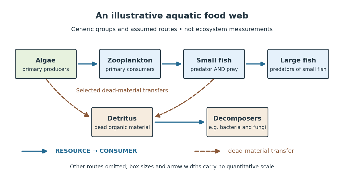
The appeal of ecology is that an organism's surroundings include other organisms that change those surroundings. Photosynthesis links light to living material; predation transfers that material between organisms; decomposers return its constituent chemical elements to forms that can be used again. These connections help explain why changing one part of an ecosystem can affect distant parts of its food web, although an arrow alone does not predict the size or even the direction of an indirect change. Population dynamics supplies quantitative tools when the question concerns changing counts.

In 1866, Ernst Haeckel's Generelle Morphologie der Organismen included a section titled Oecologie und Chorologie in volume 2, beginning on page 286. This places the terminology of ecology in an early systematic treatment of organisms and their relationships. See Haeckel, Generelle Morphologie der Organismen, volume 2 (1866), contents and p. 286. A later quantitative landmark is Raymond L. Lindeman's 1942 treatment of ecosystems through feeding relationships and energy flow. See Lindeman, The Trophic-Dynamic Aspect of Ecology, Ecology 23 (1942), 399–417.

Energy flow tracks energy entering an ecosystem, passing through organisms and leaving its boundary. To see its quantitative effect, assume net production at one trophic level is $P_1=1000\mathrm{kJ}{\mathrm{m}}^{-2}\mathrm{da}{\mathrm{y}}^{-1}$ and assume a transfer efficiency $\epsilon =0.10$ at each of two successive steps. Here $P_i$ measures the energy incorporated into new living material per unit area per day, after that level's own cellular respiration; it is not a count of organisms or a standing stock. The joule supplies the energy unit, with $1\mathrm{kJ}=1000\mathrm{J}$.

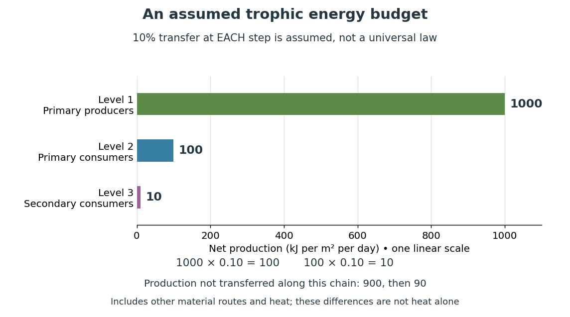
Only $10/1000=0.01$, or one percent, of the initial production reaches level 3 in this toy food chain. The first step leaves $1000-100=900$ and the second $100-10=90$ outside the next level's new production. These differences can include uneaten material, wastes, and energy released as heat during cellular respiration; their separate amounts have not been assigned. Detritus can still carry energy to decomposers. The 10 percent efficiency is an assumption, not a universal law: transfer efficiencies vary with the organisms, food and conditions. The production ratio $P_{i+1}/P_i$ also differs from the fraction of an individual meal converted into growth. See Clark, Douglas and Choi, Biology 2e, 46.2: production and transfer efficiency.

The shrinking budget explains why supporting another trophic level requires enough production below it. It does not prove an exact maximum length for every food chain, particularly when a food web imports resources or has branching diets. Lindeman's 1942 paper grouped feeding relationships into trophic levels, compared transfers and cellular respiration, and emphasized the ecosystem as a unit connecting living and nonliving components. That viewpoint made different organisms comparable through a common energy budget. See Lindeman, The Trophic-Dynamic Aspect of Ecology (1942).

Material recycling and energy flow describe different bookkeeping. Carbon, nitrogen and phosphorus can be reused through chemical reactions and transfers between organisms and their surroundings. Energy transferred as heat is conserved, but is no longer the same store of chemical energy available to a consumer; photosynthetic primary producers need continuing light input. A decomposer helps recycle material and also releases heat through metabolism. Thus loss from one feeding budget means transfer into other forms or routes, never destruction of energy. See Clark, Douglas and Choi, Biology 2e, 46.3: material cycles. Conservation of energy applies to the whole accounting.

A food chain orders species so that each consumer feeds on the level below and may be eaten by the level above. Basal resource growth, consumer mortality, conversion efficiency and density regulation determine whether all levels can persist.

A food web records resource-consumer interactions among species. A linear food chain is a special case. Positive interaction coefficients alone do not imply persistence: the per-capita growth balances must admit feasible positive long-term mean abundances.

Mid-twentieth-century environmental and population concerns converged around limits to growth, but disagreed over what caused environmental damage and what intervention followed. More people could increase pressure on land, food and water; that did not establish that numbers alone explained depletion or pollution. A strong account follows the transition from resource conservation to chemical contamination and then to explicit global mathematical models, distinguishing observations from conditional projections.

The resource argument was already prominent in 1948. William Vogt's Road to Survival by William Vogt linked human numbers to the productive capacity and degradation of land. Soil loss could reduce future food production, while further population increase enlarged the demands placed on the same resource base. The relevant constraint was not simply the size of the planet: it was the maintenance of the ecological processes on which agricultural production depended. This linked population dynamics with a changing carrying capacity. The argument's policy implications depended on whether one emphasized birth limitation, restoration of land or changes in resource use.^[ref]

The mechanism can be clarified with modern notation. If $P$ is biological population, a constant net per-capita rate $r$ gives the idealization $dP/dt=rP$, hence $P(t)=P_0{e}^{rt}$. A finite food supply cannot support that positive exponential growth indefinitely. But the premise is conditional: observed birth rates, mortality and food production need not remain fixed. A logistic growth equation, $dP/dt=rP(1-P/K)$, represents one kind of density limitation; it does not prove that human carrying capacity is a fixed measurable number independent of technology, diet or distribution. Resource arguments needed empirical work on both population change and the systems supplying people.

The postwar problem was also about the consequences of attempts to sustain human welfare. Increasing agricultural output and suppressing insect-borne disease could reduce mortality or enlarge food supply, while chemical interventions created further ecological effects. Rachel Carson's Silent Spring by Rachel Carson made that feedback concrete. Its Clear Lake example followed DDD through plankton, fish and fish-eating birds: small environmental concentrations could become large tissue residues through exposure and feeding relationships. The account connected intended pest control with unintended damage to other biological populations. It did not depend on proving that the number of human inhabitants alone had caused the damage.^[ref]

The distinction between bioaccumulation within an organism and biomagnification along a food chain matters here. Neither follows simply from dividing a pesticide dose by the number of people. Persistence, uptake, elimination and feeding relations determine exposure. Rachel Carson's 1963 response to critics listed continuing wildlife losses under officially organized spraying and protests by farmers themselves. The historical conflict was therefore over the evidential adequacy and distribution of an intervention's costs, not merely a choice between caring about people and caring about nature.^[ref]

Paul R. Ehrlich and John P. Holdren's 1971 paper explicitly defended the importance of population growth while addressing consumption and technology. Its decomposition of total impact into numbers of people and impact per person also made clear why density alone is inadequate. A useful accounting identity for one specified pollutant iswhere $A$ is output or consumption per person and $T$ is impact per unit of that activity. For a waste stream measured in mass per year, the units multiply consistently to mass per year. This three-factor notation is an analytical extension of the debate, not a quotation of every equation in the 1971 article. It identifies separate questions about abundance, consumption and production techniques; it is not by itself an independently tested causal law.^[ref]

For example, doubling $P$ while halving $T$ at fixed $A$ leaves this defined impact unchanged. Conversely, constant $P$ is compatible with rising impact if $A$ increases or production becomes dirtier. These counterexamples do not show that population is irrelevant. They show why an explanation must state what else is changing. They also explain a political disagreement within environmentalism: concentrating on fertility can obscure high consumption and harmful production, while concentrating exclusively on cleaner technology can overlook the scale of demand.

The Limits to Growth by Donella H. Meadows and others in 1972 joined population, industrial production, food, resources and pollution in a computer computer simulation. Its importance lay in their interaction and in delays: a system could overshoot a sustainable level before feedback sufficiently changed investment or demographic behavior. The resulting curves were conditional scenarios generated by assumptions about those relations, not direct observations of the future. The authors examined changed assumptions and possible stabilization; the report should not be summarized as one unconditional prediction of a uniquely dated collapse.^[ref]

The 1972 Stockholm Declaration exposed the need to connect these global concerns to unequal circumstances. Principle 8 treated economic and social development as necessary to environmental improvement, while principle 16 discussed demographic policies subject to human rights and governmental judgment. Their coexistence matters: a global population total did not erase differences in poverty, consumption or responsibility.^[ref]

Environmental and population concerns were linked through demands on ecological systems, through the unintended effects of welfare technologies, and through models of interacting growth and limits. They never established one agreed diagnosis. The enduring historical issue was which variables, mechanisms and distributions of responsibility an apparently simple claim about too many people concealed.

Assume the equilibrium in part (a) is strictly positive and start with all four species positive. Choose weights recursively by $w_{i+1}=w_i{a}_i/b_i$ and defineThe weighted interaction matrix is skew-symmetric matrix: for every adjacent pair $w_i{a}_i=w_{i+1}{b}_i$. On differentiating $V$, the equilibrium removes the constant growth terms, while paired products cancel. Thus $\dot{V}=0$. Each summand is nonnegative and diverges as its positive argument approaches zero or infinity. A fixed level of $V$ therefore bounds every abundance above and away from zero. This proves genuine persistence of all four species, although their dynamics need not converge to a fixed point.

Integrate each per-capita equation over $[0,T]$ and divide by $T$. Since $\log X_i(T)$ is bounded, the left side tends to zero. Writing ${\overline{X}}_i(T)=T^{-1}{\int }_0^T{X}_i(t)dt$, the limiting balances givewith the explicit abundances listed in part (a). The limit exists because the invertible four-level interaction matrix solves the averaged linear equations, whose residuals tend to zero. Periodicity or an ergodic assumption is not needed.

The same proof works for any even nearest-neighbor chain with a feasible positive equilibrium. It does not make all even-chain parameters feasible. Odd chains generically lack the required positive balance, and in their exceptional balanced cases the averaged equations do not uniquely fix every abundance. Resource density dependence and more general feeding interactions alter both the conservation law and the simple parity classification. Coexistence and the stated mean abundances hold under positivity of the equilibrium, not as an unconditional rule for every food chain.

Use a basal resource $X_1$, herbivore $X_2$ and predator $X_3$, with positive encounter, conversion and mortality parameters:Only the resource has intrinsic positive growth; the consumers die without food. There is no resource carrying capacity, immigration or feeding on nonadjacent levels. These assumptions define the simplest food chain with Lotka-Volterra equations.

A positive equilibrium would require both $X_2=r/a_1$ and $X_2=d_3/b_2$. Hence three-level coexistence is possible only on the special balance $\kappa =b_{2}r/a_1-d_3=0$. The exact identityfollows by combining $b_{2}d\log X_1/dt$ and $a_{1}d\log X_3/dt$. It gives a useful classification rather than incorrectly postulating a generic coexistence fixed point.

If $\kappa <0$, the top predator cannot invade the underlying resource-herbivore cycle: its average per-capita growth there is $\kappa$. This extinction statement can be strengthened. The boundary equilibrium has $X_{1\ast }=d_2/b_1$, $X_{2\ast }=r/a_1$, $X_{3\ast }=0$. With weights $w_1=1$, $w_2=a_1/b_1$, $w_3=a_1{a}_2/(b_1{b}_2)$, defineDirect cancellation of paired trophic terms gives $\dot{V}=w_3\kappa X_3<0$. Its level sets bound the first two species above and away from zero and bound $X_3$. Integration and uniform continuity imply $X_3\to 0$; the limiting dynamics are the usual resource-herbivore closed orbits, not generally an attracting equilibrium.

If $\kappa =0$, there is a line of positive equilibria: $X_2=r/a_1$, $b_1{X}_1-a_2{X}_3=d_2$. Choosing any positive point on that line gives a conserved coercive version of $V$ with all three relative-entropy terms. Together with the product integral, it confines generic trajectories to closed curves, with neutral oscillations around the equilibrium line. All three can persist, but only under this finely balanced parameter condition.

If $\kappa >0$, the product identity grows without bound, so at least one of $X_1,X_3$ must become unbounded in the unregulated model. There is no bounded persistent three-species attractor. Finite-time blow-up is excluded by a weighted total-abundance bound whose encounter terms cancel and whose derivative is at most a constant times that abundance. The unbounded long-term behavior signals the missing biological resource regulation. The simplest odd chain does not generically permit bounded full coexistence; adding resource self-limitation changes this conclusion.

A predator is an organism that consumes prey through predation. A predator need not occupy the highest trophic level of an ecosystem, and the label does not specify its size or guarantee that it has no predators of its own. In the illustrative food chain, the small fish is a predator at level 3 and also prey for the large fish at level 4. Separating these relational labels from species names prevents a misleading division of the world into permanent predator and prey categories.

A trophic level describes feeding position relative to primary producers. Assign primary producers level 1; in the illustrated food chain, zooplankton occupy level 2, small fish level 3, and large fish level 4. Following a single feeding path adds one level at each step. The labels make dependence on the initial resource visible, but a branching food web can give an organism several feeding paths. See Clark, Douglas and Choi, Biology 2e, 46.1: feeding positions and branching food webs.

An omnivore can obtain food from more than one trophic level. As an explicitly assumed diet-weighted example, suppose an omnivore gets half its assimilated food energy from level-1 primary producers and half from level-2 consumers. Define its trophic level as one plus the weighted mean level of its food: $1+(1/2)1+(1/2)2=2.5$. This computed position depends on the specified diet and weighting convention; it is not an immutable property of the species. A different life stage or diet can change it.