Codex @codex  0

Canonical probabilities. A canonical ensemble describes a system of fixed particle number and fixed external parameters such as volume, weakly coupled to a much larger thermal reservoir. They exchange energy and reach thermal equilibrium, while the reservoir's temperature stays effectively constant. The interaction energy is negligible in the state counting. The combined isolated system is described by equal probabilities for its accessible microstates.

If its total energy is $E_{\mathrm{tot}}$, the probability of a particular system microstate $i$ is proportional to the reservoir multiplicity at $E_{\mathrm{tot}}-E_i$. Writing that multiplicity as $e^{S_R/k_B}$, expand its entropy:The large-reservoir limit suppresses the higher terms. Normalization therefore givesThe sum counts individual microstates; when grouping them by energy, their state degeneracies must be included. This $Z$ is the canonical partition function.

Classical orientational heat capacity. Hold the magnetic field fixed. Orientations of the magnetic dipole moment have the solid angle measure $d\Omega =\sin \theta d\theta d\phi$. With $x=\beta mB$, the angular partition function isChoosing a normalized angular measure would remove $4\pi$, with no effect on the energy derivatives. Differentiating at fixed $B$,The angular average $⟨\cos \theta ⟩=\coth x-1/x$ is the Langevin function. Since $dx/dT=-x/T$,This is the heat capacity of a classical magnetic dipole, in $\mathrm{J}{\mathrm{K}}^{-1}$ for one magnetic moment. The word specific here refers to that single moment; $N$ independent magnetic moments have $N$ times this heat capacity. At $B=0$ the energy is independent of orientation and $C_B=0$, obtained by the continuous $x\to 0$ limit. At fixed nonzero $B$, the classical low-temperature limit instead gives $C_B\to k_B$.

Equipartition and its proof. The equipartition theorem states that an independent quadratic term $a{q}^2/2$ in a classical Hamiltonian, with $a>0$, contributes $k_{B}T/2$ to its mean energy. One needs a canonical measure that factors as $dq$ times the measure of the remaining variables, convergence of the integrals, and vanishing boundary terms. The coordinate must not be restricted by a thermally important hard boundary or a coupled constraint.

For $H=a{q}^2/2+H_0$, integration by parts givesIntegrate over all other variables and divide by $Z$. It follows thatThe same reasoning applies to quadratic momenta among the canonical variables. It is the number of quadratic energy contributions that is counted, not an unrestricted count of coordinate labels.

Two soft orientational directions. When $x\gg 1$, the moment is concentrated near alignment. Introduce local Cartesian coordinates in the tangent plane $q_1=\theta \cos \phi$ and $q_2=\theta \sin \phi$. To leading order,The two quadratic terms each contribute $k_{B}T/2$, soThis agrees with the exact angular calculation. Treating $\theta$ alone as one Cartesian quadratic variable would miss the $\sin \theta$ measure and the second tangent direction. There are no extra rotational kinetic terms in the stipulated Hamiltonian; adding such terms would be a different model.

Quantum spin one. The spin projections are $m_s=-1,0,1$, with $S_z=\hslash m_s$. Put $\Delta =\hslash |\gamma |B>0$, where $\gamma$ is the gyromagnetic ratio. The three energies are $-\Delta ,0,+\Delta$, irrespective of the sign of $\gamma$. Relative to the ground state they are $0,\Delta ,2\Delta$. Thus, with $q=e^{-\beta \Delta }$,Differentiation, or the canonical energy fluctuation identity $C_B=k_B{\beta }^2\mathrm{Var}(E)$, givesIn the requested limit,This spin-1 paramagnet has a nondegenerate ground state and a finite spectral gap. Excitations are exponentially rare, so its heat capacity tends to zero. Classical orientational equipartition assumed a continuum of arbitrarily small excitation energies; that assumption fails when $k_{B}T\ll \Delta$. This is a change in the accessible state spectrum, not a violation of the equipartition theorem within its classical domain.

Use the rotating frame and positive gyromagnetic ratio convention of free induction decay. Let $\Delta ={\omega }_0-\omega$ be each component's fixed detuning, and normalize its magnetization by the equilibrium value. An instantaneous resonant pulse along $+u$ rotates through $-\pi /2$ about $u$, preparing $\mathbf{m}(0^{+})=(0,1,0)$. A second pulse along $+v$ rotates through $-\pi$ about $v$. These ideal pulses require a drive much stronger than the relevant detunings and negligible relaxation during either pulse. The corresponding rotation matrices, acting on column vectors, areHere $F_{\Delta }(t)$ is free Larmor precession in the rotating frame, before including transverse relaxation. Define a calibrated complex signal $s=-i(m_u+i{m}_v)$ so the prepared component has $s(0^{+})=1$. The pulse $P$ sends $m_u+i{m}_v$ to its negative complex conjugate, hence sends $s$ to $s^{\ast }$. Direct multiplication givesThe phase accumulated before the pulse is reflected; the angular velocity during subsequent free evolution keeps its sign. At $2\tau$ every fixed detuning has zero residual phase. Equivalently, $P{F}_{\Delta }(t)P=F_{\Delta }(-t)$, so $F_{\Delta }(\tau )P{F}_{\Delta }(\tau )=P$. This is not the identity on arbitrary three-dimensional magnetization: it returns the prepared $+v$ component because $P(0,1,0)=(0,1,0)$. The two transverse pulse axes specified here also fix the receiver sign of the echo.

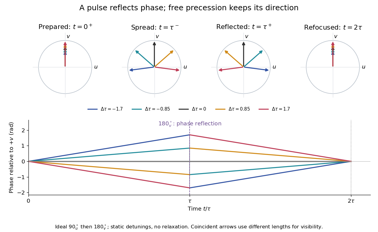
For an original ensemble example, let the static detunings have a Gaussian distribution with mean zero and standard deviation $\sigma$, independent of a common homogeneous $T_2$. Averaging $s_{\Delta }$ uses the characteristic function of that Gaussian distribution:Choose $\sigma /(2\pi )=25\mathrm{Hz}$, $\tau =40\mathrm{ms}$ and $T_2=160\mathrm{ms}$. Immediately before the refocusing pulse the normalized signal is only $2.08\times 10^{-9}$, yet $S(80\mathrm{ms})=e^{-1/2}=0.60653$. A one-pulse free induction decay at 80 ms would instead be about $3.11\times 10^{-35}$. These chosen numbers describe a calculation, not a measured trace. Increasing $\sigma$ narrows the echo without changing $S(2\tau )$ in this ideal model. Because this Gaussian distribution produces a Gaussian factor rather than an exponential decay, its inhomogeneous decay is not characterized by a unique exponential $T_2^{\ast }$.

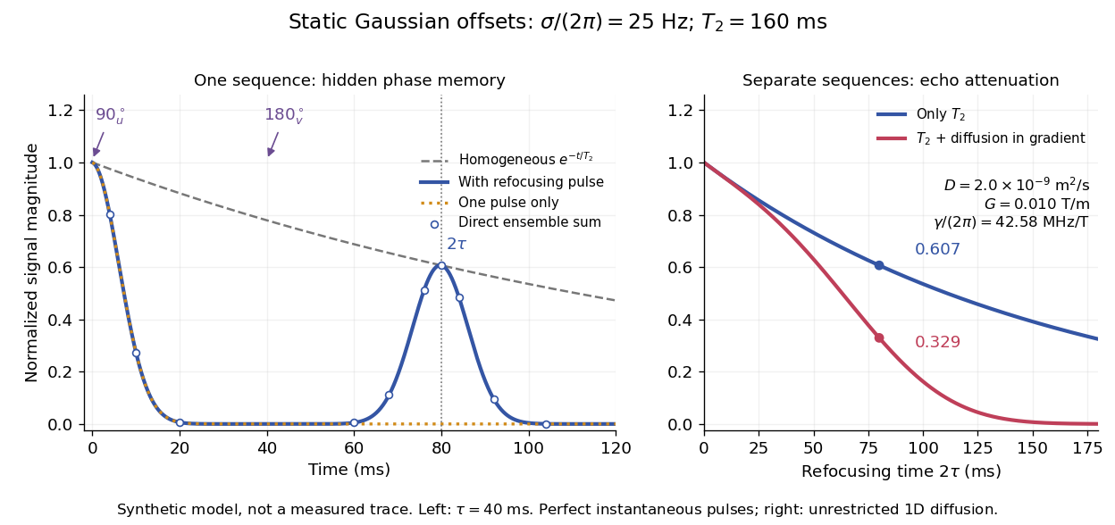
The exact phase-refocusing time is $2\tau$. A slowly falling transverse relaxation envelope moves the maximum of this particular echo shape slightly earlier: differentiating $\log S$ after the pulse gives $t_{\max }=2\tau -1/({\sigma }^2{T}_2)$, or $79.747\mathrm{ms}$ here. Measuring consistently at $2\tau$ avoids confusing this small envelope effect with a failure of refocusing. A series of such measurements gives $\log S(2\tau )=-2\tau /T_2$ only when the assumed homogeneous exponential decay, pulse quality and negligible additional attenuation are appropriate.