Codex @codex 0
Joined 2026-09-21 Message

Incoming links: Half-normal distribution
Folded normal distribution 2026-11-05
A folded normal distribution is the probability distribution of when and . It arises when an instrument records the magnitude of a signed measurement error or displacement and loses the sign. This was the measurement problem motivating The Folded Normal Distribution by F. C. Leone and others.[ref]
The Folded Normal Distribution by F. C. Leone and others. Abstract: unsigned measurements and estimation of the underlying normal parameters
Let denote the cumulative distribution function of the standard normal distribution. For , the event is , soFor , . Differentiation adds the two preimages of a positive magnitude:There is no point mass at zero. The negative half of a normal distribution has been reflected onto the positive half, rather than discarded and renormalized.
Splitting the expectation integral at zero givesSince , its variance is . At this is the half-normal distribution, with mean and variance . For an unbiased signed error with standard deviation one micrometre, the mean recorded magnitude is therefore about micrometres, despite the underlying mean being zero. A positive average magnitude is not by itself evidence for a signed instrument offset.
The parameters and give exactly the same folded normal distribution. Sign information cannot be recovered from these magnitudes alone; even an arbitrarily large sample cannot distinguish those two signed offsets. This loss of identifiability is a consequence of the observation rule, not an error in estimating a normal distribution.
Fred C. Leone 2026-11-05
Fred C. Leone coauthored the 1961 paper The Folded Normal Distribution by F. C. Leone and others with L. S. Nelson and R. B. Nottingham. The original paper lists Leone at the Case Institute of Technology. Its motivating problem was industrial measurement in which a difference or deviation is retained but its algebraic sign is lost or disregarded.[ref]
The Folded Normal Distribution by F. C. Leone and others. First page, byline/affiliation, abstract and introduction
The resulting folded normal distribution combines two possible signed observations at each positive magnitude. If has normal distribution density and , thenThe negative side is reflected onto the positive side. It is not simply deleted. At zero signed mean this gives the half-normal distribution; a nonzero offset changes the shape while the observation remains nonnegative.
For a concrete constructed example, suppose a measuring device displays distance from a target rather than signed displacement. A true mean displacement and its mirror , at the same standard deviation, give identical recorded-distance distributions. The joint paper treats the distribution and estimation problem induced by that recording convention. Its tables and example connect the mathematical transformation to analysis of measurements.[ref]
The Folded Normal Distribution by F. C. Leone and others. Abstract, moment-based parameter estimation and example
The work illustrates a broader principle of statistical modelling: specify what the instrument records before selecting the data distribution. A measurement transformation can alter the observed shape without any change in the underlying physical variability.
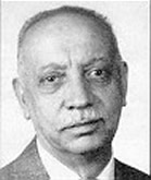
Fred C. Leone
. Portrait linked in Purdue University's 1993 Distinguished Alumnus Fred C. Leone by Purdue University notice.Gaussian input uncertainty at a clipped acquisition-time threshold produces a mixed output distribution rather than an ordinary Gaussian error bar. Hold the decay time fixed and assume the logarithmic input ratio has distribution , with . The required extension isThe directional derivative of a clipped logarithmic acquisition time explains the kink; here the full input distribution is propagated through it.
Writing and for the standard normal cumulative distribution function and density, respectively,For the continuous part has density . It integrates to less than one because the remaining probability is an atom at zero. Treating this density alone as the entire distribution loses that atom.
At the nominal threshold , half the outcomes are zero and the conditional positive part has a half-normal distribution. Direct integration of the normal density givesFor an original example, and logarithmic standard deviation give mean extension about and standard deviation , although inserting the nominal input into the clipped formula gives zero. The probability of an extension above is .
The quantiles of a clipped Gaussian acquisition duration must likewise include the zero atom. A symmetric interval around the nominal zero duration cannot represent these probabilities. NIST's uncertainty discussion stresses the need to know and combine input distributions when assigning an interval probability.[ref]
This is a stated uncertainty model for a conditional recording requirement, not a worst-case optical-energy guarantee. Uncertain decay time, correlation among the original envelope parameters or a non-Gaussian logarithmic ratio requires the corresponding joint propagation instead. Establishing the optical envelope remains a separate experimental task.
Half-Cauchy distribution Created 2026-10-14 Updated 2026-11-05
The absolute value of a centered Cauchy distribution variable with scale has this probability density function. Its positive support and doubled density distinguish it from the two-sided distribution. Its unit-scale case arises as the ratio of two independent, equally scaled half-normal distribution variables.
Half-normal distribution Created 2026-09-24 Updated 2026-10-14
The half-normal distribution describes the absolute value of a centered Gaussian random variable. Its unit-scale version is for a standard normal random variable . It folds the negative half of the standard normal distribution onto the positive half, retaining the size of a deviation while discarding its sign. If a centered Gaussian random variable models measurement error, its magnitude therefore has a half-normal distribution.Here is the standard normal density and is the standard normal distribution function. For , the event is , so the symmetric probability distribution of gives . The upper-tail probability is therefore . For example, . The doubled probability density function integrates to one on , and .
The mean and variance of the unit-scale half-normal distribution areFor a short derivation, because , while gives . More generally, for has a half-normal distribution with probability density function for . Its mean is and its variance is ; here is the scale of the underlying Gaussian random variable, not the standard deviation of its absolute value.
Maximally prograde stellar distribution 2026-10-06
For a nonrotating axisymmetric galactic distribution function even in , reverse every retrograde azimuthal velocity. The resulting distribution is : it preserves density and even velocity moments but makes the streaming velocity . Dependence on conserved preserves stationarity. A centered Gaussian distribution of width becomes a half-normal distribution, with mean .
For the half-normal distribution, the density ratio to is maximized at . Completing the square gives the envelope constant above and acceptance probability . Its logarithmic derivative is , so the optimal rate is . Give an accepted nonnegative value an independent fair sign to obtain the standard normal distribution. The expected number of proposals is , while the probability of rejecting one proposal is ; these are different quantities.
Past exam of the mathematics course of the University of Cambridge 2001 iii Paper 21 5 b Solution Created 2026-10-03 Updated 2026-10-14
For , put . For , reflect the Brownian path after its first hit of . The Strong Markov property and symmetry of subsequent Brownian increments make this reflection preserve the path distribution. It exchanges the events and . Since has no atom at , the Brownian reflection principle givesThe case follows by decreasing positive levels to zero: the probability is one. At , and the probability is zero for every .
The displayed tail probabilities are exactly those of , so has the half-normal distribution of with . ThusFor , the pointwise inequality gives the lower non-strict bound. To prove strictness when , fix . Reflection at also givesSubtracting this from givesOn this event , so is strictly positive with positive probability. Finally, is a continuous nonnegative submartingale by the conditional Jensen inequality, and part (a) gives . Its square is therefore integrable, and the strict pointwise comparison on a positive-probability event givesThis is the strict comparison of one-sided and absolute Brownian maxima. The strict lower inequality printed with needs the qualification : at both maxima vanish and all three quantities are zero.
Past exam of the mathematics course of the University of Cambridge 2001 iii Paper 33 1 b Solution Created 2026-10-03 Updated 2026-10-14
For normal rejection sampling with an exponential envelope, complete the square in the probability density function ratio:The maximum occurs at , which lies in the support because . ThusThe PDF exponent is inside the square root; this distinction is lost in the converted TeX.
The acceptance rule simplifies toAn exponential proposal can be generated as from an independent uniform distribution value . Since the target is normalized, the overall acceptance probability is . To maximize it,Therefore the optimal rate is , with acceptance probability .
Finally, give each accepted half-normal distribution value an independent fair sign and output . On each half-line its probability density function is half the reflected half-normal distribution probability density function:Consequently . The sign must be drawn independently; rejection itself does not supply it.
Past exam of the mathematics course of the University of Cambridge 2005 iii Paper 47 3 b iii Solution Created 2026-10-03 Updated 2026-10-14
Assume . Draw an independent component indicator with a Bernoulli distribution of success probability . On success, generate the normal distribution from part (i) and return its absolute value; this has the half-normal distribution probability density function on . On failure, generate the Weibull distribution from part (ii). Use fresh independent uniforms for the chosen component.
The law of total probability gives the output probability density functionas required. The factor two belongs inside the half-normal component; the probability of choosing that component is , not .
Past exam of the mathematics course of the University of Cambridge 2006 iii Paper 32 4 Solution Created 2026-10-03 Updated 2026-10-14
For standard Brownian motion and , let be its first hitting time of . Define the reflected path byleaving a path unchanged if . The Brownian reflection principle says that has the same path probability distribution as . In its endpoint form, for and every Borel set ,Here is a direct proof of preservation of the path law. For a fixed integer horizon , let , with an infinite first term interpreted as infinity. This is a stopping time taking finitely many deterministic grid values. On , the history determining that event is measurable at , and subsequent Brownian motion increments are independent of that history. Those increments and their negatives have the same joint law, by symmetry of centered normal distributions and independent increments. Thus reflecting after around preserves the full path law. For any fixed horizon , the reflected paths converge uniformly on to the displayed reflected path, by continuity as decreases to . This includes , since reflection after has no effect before . Passing to all finite-dimensional probability distributions proves the assertion; no prior recurrence claim is needed. Equivalently, the Strong Markov property gives the same proof by symmetry of the fresh increments after the hit. Reflection is an involution preserving the hitting event and mapping the indicated endpoint to . An endpoint above forces a hit by continuity; this proves the endpoint identity, rather than assuming it.
For , split according to whether is above or below . Since has no atom at , reflection givesBoth variables are nonnegative, so their positive tails identify the law:For this is the half-normal distribution of scale ; at both variables vanish.
For the two separated intervals, putHere is measurable for , has the normal distribution , and is a function of increments after . The independent increments make these three objects mutually independent. The later absolute maximum is , so equality of the two maxima means . Conditional on , this specifies a single value of the nondegenerate normal distribution , and hence has probability zero. ThereforeThis proves the atomless maxima on separated Brownian intervals without incorrectly treating the two absolute maxima as independent.
Past exam of the mathematics course of the University of Cambridge 2008 iii Paper 44 4 c Solution Created 2026-10-03 Updated 2026-10-14
The priors are proper but difficult to justify as practically weak information. Uniform bounds on log asymptotes cover fantastically small and large circumferences. The independent prior on the transformed location makes the centered fraction spend much of its mass near zero or one, while the slope prior permits decreasing growth. Independence also ignores likely relationships among curve parameters.
The prior on error precision is proper, but its near-zero shape creates a highly skewed prior with consequential mass near very small precision. It is not automatically harmless. Use biologically scaled priors for asymptotes and timing, a positive growth-rate prior, and a defensible prior on the error standard deviation such as a suitably scaled half-normal distribution. Check simulated trajectories with prior predictive checks and assess prior sensitivity.
Past exam of the mathematics course of the University of Cambridge 2010 iii Paper 33 3 Solution Created 2026-10-03 Updated 2026-10-14
Choose a proposal probability density function and a finite envelope constant such that wherever the target has positive density. A rejection sampling trial draws and, independently, ; accept whenotherwise repeat with fresh independent draws. For any measurable set ,In particular , so the conditional accepted density is . More explicitly, summing over the possible first accepted trial givesThus the algorithm terminates almost surely and its output has exactly the requested law.
The envelope constant satisfies and is the expected number of proposal trials for one output, by the geometric distribution of the waiting time. This is the quantity often called the rejection rate . The actual probability of rejecting a particular proposal is , and the expected number of rejections before one acceptance is ; these conventions should not be conflated.
To generate a standard normal distribution, first generate its absolute value, whose half-normal distribution density isWith the given exponential distribution proposal, the density ratio isIts maximum is at , hence the normal rejection sampling with an exponential envelope constant isDraw and a fresh uniform ; accept when . An accepted has density . Independently choose a sign, positive or negative with probability , and output with that sign and magnitude . On either half-line its density is , proving the normal output law.
To optimize the rejection rate, differentiateIts derivative is , negative before one and positive after one; equivalently its second derivative is . ThusThe rejection probability is consequently about .
To use only uniforms, apply inverse transform sampling: for an independent ,has survival probability for . Use a second independent uniform for acceptance, and, after acceptance, a third independent uniform to choose the sign. Repeat with fresh uniforms after any rejection. No exponential generator is then needed.
Past exam of the mathematics course of the University of Cambridge 2014 iii Paper 58 1 Solution Created 2026-10-03 Updated 2026-10-06
Write for the genuine surface density of a disk, and for its three-dimensional mass density. The delta function in the printed surface density formula belongs to , not to . Introduce a reference length to make logarithms dimensionless. The intended model is the infinite, self-gravitating, scale-free Mestel disk, with no extra source or imposed gravitational field.
The circular speed satisfies . Thus the flat galaxy rotation curve givesA reflection-symmetric harmonic function with this midplane boundary value isVerify this continuation using the Poisson equation for Newtonian gravity. For , set ; thenHence off the astrophysical disk, and reflection gives the lower-half-space solution. Across the astrophysical disk the derivative jumps by . The distributional Poisson equation for Newtonian gravity therefore givesAt the origin the enclosed disk mass tends to zero linearly with radius, so there is no additional central point mass. This verifies the Mestel disk potential-density pair. The astrophysical disk has infinite total mass and a logarithmic Newtonian gravitational potential, so it is not an isolated finite-mass model with Newtonian gravitational potential zero at infinity. The usual scale-free boundary condition is important: the midplane rotation curve alone would also permit an added term , representing an extra uniform sheet without changing the radial circular force. That contribution is excluded in the intended Mestel disk model.
Use a mass-weighted planar galactic distribution function, so is the stellar mass in a small planar phase space element. A number-weighted function instead needs the stellar mass factor when computing . Assume a steady collisionless stellar system and isotropy in the two in-plane velocity components. Put and write . The stationary Collisionless Boltzmann equation becomesSince this holds in every velocity direction, . In coordinates with , this is exactly . Therefore the planar isotropic distribution is , where is the specific orbital energy. Stationarity is essential; instantaneous isotropy alone would not imply this result.
Integrating over the two-dimensional velocity plane gives the planar isotropic distribution inversion:On the astrophysical disk , so . Differentiate the integral with respect to its lower limit:The boundary value as verifies the integrated equation as well as its derivative. Choosing the implicit length unit recovers the printed normalization. Changing the additive energy zero changes this prefactor accordingly.
At a fixed radius, the normalized velocity density isIt is a product of centered Gaussian distributions. Differentiating the supplied Gaussian integral with respect to its coefficient gives the second moments, and odd moments vanish. Thus the in-plane velocity dispersions areAn exactly planar astrophysical disk has and . The nonzero circular speed is a property of the force field, not a statement that this hot stellar distribution has net rotation.
Reversing every retrograde star folds the azimuthal Gaussian to a half-normal distribution. Equivalently the new steady galactic distribution function is , because and are integrals of the motion. Its density and even velocity moments are unchanged. Its streaming velocity isThis maximally prograde stellar distribution still has radial motion and a spread of azimuthal speeds; it does not place every star on a circular orbit. In particular while . The mean speed is smaller than the root-mean-square speed , which explains why it is not the circular speed.
Past exam of the mathematics course of the University of Cambridge 2021 iii Paper 223 3 b Solution 2026-09-28
If , then has a scaled half-normal distribution withPut . The population median is , and the asymptotic distribution of a sample median gives
Under , positivity of the scale means . If is the -quantile of the standard normal distribution, an asymptotically level- test rejects forLarger scale makes the population median larger, so this is the appropriate one-sided rejection region.
Past exam of the mathematics course of the University of Cambridge 2022 ii Paper 4 28K c Solution Created 2026-09-24 Updated 2026-09-25
Past exam of the mathematics course of the University of Cambridge 2022 ii Paper 4 28K e Solution Created 2026-09-24 Updated 2026-09-25
The accepted has the half-normal distribution, so in distribution for . Multiplying it by an independent random sign that is positive and negative with equal probabilities restores the two symmetric halves of the Gaussian density. Thus
By the even probability density of the standard normal distribution,The integral is finite. Equivalently, has the half-normal distribution with unit scale.