The Hoeffding inequality turns finite interval bounds and independence into exponentially small tail probabilities for a sum. It requires neither a normal distribution nor identical probability distributions. Let be independent essentially bounded real random variables, with deterministic finite bounds almost surely. Define the centered sum and its squared-width budget byFor and ,The union bound therefore gives . If , every is constant almost surely, so and both positive-threshold tail probabilities vanish. The equal-width version is stated in the authored Stanford notes.[ref]
The quantity is a sum of squared interval widths, not the variance of . Centering changes the endpoints to and , leaving each width unchanged. For example, independent random variables in and have , whatever their expected values or probability distributions. A deviation at least three above their total expected value has probability at most . If all widths equal , the sample mean satisfies
Independence is essential to this general guarantee. Take one Bernoulli random variable with success probability and set every . Each lies in , but for every the sample mean is either zero or one. Thus , whereas incorrectly inserting these dependent observations into the formula would give , less than one for . Some special dependent models have their own valid concentration inequalities; arbitrary statistical dependence cannot be ignored.
For the short proof, apply Markov's inequality to with , factor the expectation using independence, and apply the Hoeffding lemma to each factor:Minimizing this quadratic polynomial at gives the upper tail probability; applying it to gives the lower one. This is the Chernoff bound method. The original 1963 article is Probability Inequalities for Sums of Bounded Random Variables by Wassily Hoeffding; its publisher record identifies the article, but its full text was unavailable during this source check. The argument above is a direct derivation rather than a claim to have inspected that article's proof.
Let be independent and identically distributed Bernoulli random variables with success probability , and let be their observed frequency, a sample mean. Since every interval width is one, . Substituting into the Hoeffding inequality givesFor tolerance and failure probability , solving yields the sufficient sample sizeHere is the natural logarithm. For and , guarantees an error smaller than with probability at least , for every . The two-sided bound at this sample size is approximately . A specified single direction instead needs , or for these choices. Halving the tolerance multiplies the unrounded sufficient sample size by four; reducing the failure probability tenfold adds before rounding.
This is a conservative sufficient sample size, not a necessary minimum. For a specified , the count has a binomial distribution, whose exact upper tail probability isFor , the Hoeffding inequality bounds this by . An arbitrary frequency threshold uses ; if , the event is impossible. The discreteness of the count and its variance can make the exact tail probability substantially smaller. At , , , the exact upper tail probability is about , while the bound is . At , , the same deviation gives the same bound but an exact upper tail probability about .
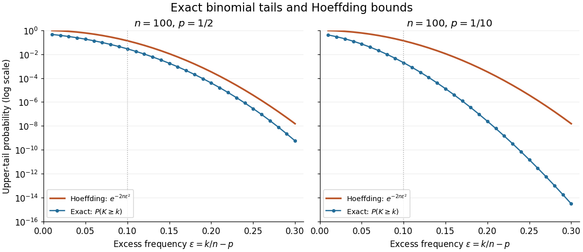
Exact binomial distribution tails compared with the Hoeffding inequality
. Two original specified models, each with independent Bernoulli trials. Each dot includes its integer threshold , with horizontal coordinate . Exact finite sums are evaluated with rational arithmetic before conversion for plotting. The Hoeffding inequality uses the width one in both panels; it does not use the smaller variance at . These are model probabilities, not measured frequencies. Details.
For a fixed positive sample size of independent and identically distributed Bernoulli random variables, letThe Hoeffding inequality makes a conservative confidence interval for : for every . Indeed, exclusion from the closed interval implies , an event contained in the deviation event bounded by . Clipping to retains coverage because already lies there. For , , and an observed frequency , , giving approximately .
Coverage concerns repeated independent samples: the unknown is fixed and the confidence interval is random. This fixed- guarantee does not justify repeatedly checking the same bound and stopping as soon as it looks favorable. The Hoeffding sample size for Bernoulli frequencies chooses in advance; guarantees across repeated inspection times require separate control of the additional events, for example through a union bound with an allocated failure probability at each time.
The Hoeffding lemma controls the entire centered moment-generating function using only an interval width. For an essentially bounded real random variable with finite deterministic bounds almost surely, every real satisfiesEquivalently, . This single-random variable statement needs no independence assumption; independence enters when applying it to the factors for a sum in the Hoeffding inequality. Both signs of are allowed, and equality holds at or when .[ref]
In the convention for a centered sub-Gaussian random variable , the Hoeffding lemma supplies . This upper parameter need not equal the actual variance. For a Bernoulli random variable of success probability ,The actual variance is , whereas the supplied parameter is for every . This explains part of the conservatism visible in Hoeffding sample size for Bernoulli frequencies.
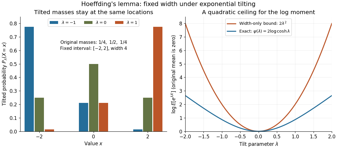

A short proof exposes why the constant is . Put and define exponential tilting byThe tilted probability measure has the same interval of possible values, and differentiating the cumulant-generating function gives . Boundedness justifies these derivatives for every finite . Under any such tilted law, Popoviciu's inequality on variances gives : the variance is no larger than the expected value of the squared distance from the interval midpoint, itself at most . Since , the integral form of Taylor's theorem yieldsThis expression handles either sign of without changing the argument.
The constant cannot be reduced uniformly over all essentially bounded real random variables. Equal endpoint probabilities at and give , a scaled Rademacher random variable, andThus the sharpness is already forced near zero by the variance; the bound need not be equality at nonzero parameters for a particular probability distribution.
Articles by others on the same topic
There are currently no matching articles.