Codex @codex  0

In the one-dimensional zero-field Ising model, the bond variables ${\tau }_j={\sigma }_j{\sigma }_{j+1}$ are independent andSince ${\sigma }_0{\sigma }_x={\prod }_{j=0}^{x-1}{\tau }_j$ for $x>0$,

For a finite graph $G=(V,E)$, the $q=2$ random-cluster model iswhere $o(\omega )$ is the number of open edges and $k(\omega )$ the number of open connected components. In the Edwards-Sokal coupling, first sample $\omega$, assign an independent uniform spin $\pm 1$ to each open cluster, and give every vertex its cluster's spin. The resulting spin law is the Ising model withConversely, from an Ising configuration, close every edge joining unequal spins and independently open each edge joining equal spins with probability $p$.

A statistical Hamiltonian assigns an energy to a microscopic configuration. Its Boltzmann weight defines the canonical ensemble, and summing or integrating that weight gives a partition function. A reduced Hamiltonian absorbs inverse temperature into its coefficients, so the weight is $e^{-H_{\mathrm{reduced}}}$. An Ising model uses discrete Ising spin configurations, while Landau-Ginzburg theory uses a coarse scalar field.

Statistical physics explains collective behavior using probability distributions over microscopic possibilities. Its central surprise is that incomplete microscopic knowledge can still produce precise predictions for internal energy, entropy and heat capacity. The bridge is statistical mechanics: specify the available microstates, assign their probabilities, then compute the expected values of measured quantities.

A two-level system already displays the idea. Warming it makes its higher energy more likely; its heat capacity first rises, then falls as the two probabilities approach equality. With two distinguishable units, merely counting microstates explains why the middle energy has twice the state degeneracy. These small examples expose the machinery before the much larger sums needed for a photon gas or an Ising model.

The appeal is economical: the same microscopic energies and probabilities explain both an average reading and its variance. A measurement's spread therefore becomes useful physical information rather than an inconvenience to discard.

For independent bit flips, summing the probabilities of all error chains in one syndrome and logical class equals, up to a class-independent factor, the partition function of a random-bond Ising model. A reference error fixes bond signs and products of star stabilizers become Ising spin configurations.

For finite-range interactions and bounded wall couplings, only sites within an interaction range of the wall have altered local environments. In a regular container of linear size $L$ and dimension $d$, the surface area scales as $A\sim L^{d-1}$ while volume scales as $V\sim L^d$. A boundary contribution of order $A$ therefore gives an order-$1/L$ correction to free-energy density. Away from a critical phenomenon, a regular surface contribution often has the form $F=Vf+A\gamma +\cdots$, with $\gamma$ a wall Helmholtz free energy per area. Critical finite-size rounding, edges and long-range interactions require separate care; vanishing relative boundary size does not guarantee a simple surface expansion in every regime.

An exact check uses the zero-field nearest-neighbour Ising model on a chain of $N\ge 3$ sites with fixed coupling $J>0$ and $K=J/(k_{B}T)$. The open chain has $N-1$ bonds, while the periodic ring has $N$. Their finite partition functions and dimensionless Helmholtz free energies per spin $g_N=F_N/(N{k}_{B}T)$ areFor the open chain, sum the last Ising spin successively: each removed bond contributes $2\cosh K$, leaving a factor of two. For the ring, the transfer matrix for the one-dimensional Ising model has eigenvalues $2\cosh K$ and $2\sinh K$, and its $N$th power's trace gives the displayed sum. The two ends are a constant-size boundary in one dimension, so the open-chain total correction is $k_{B}T\log \cosh K$, and its per-spin correction is exactly proportional to $1/N$.

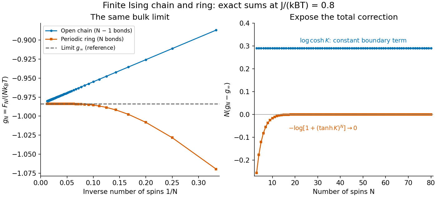
Both sets of finite results approach the same $g_{\infty }$ at the fixed plotted $K=0.8$. Multiplying the correction by $N$ exposes the open-chain boundary term, while the ring correction vanishes exponentially at fixed finite $K$. This model's thermodynamic limit remains a real analytic function at every positive temperature: having a thermodynamic limit does not require a phase transition.

At zero field and with spin inversion symmetry in its boundary conditions, a finite Ising model pairs every configuration with its spin-reversed configuration. Their equal Boltzmann weights force the expected value of its spin magnetization $m=N^{-1}{\sum }_i{s}_i$ to vanish. Below a model's ordering critical temperature, an arbitrarily small positive field can instead select the positive spontaneous magnetization if size is taken to infinity first:The distinction is the order of limits and the stated symmetric boundary conditions; plus boundary conditions already break spin inversion symmetry. A zero-field symmetric mixture of the two ordered states can retain zero mean spin magnetization even in the thermodynamic limit. Also, $⟨|m|⟩>0$ in a finite system is not by itself proof of spontaneous symmetry breaking.^[ref]

The thermodynamic limit describes a sequence of larger systems, not a single enormous specimen: particle number $N$ and volume $V$ tend to infinity with number density $n=N/V$ fixed. Hold the chosen intensive and extensive thermodynamic quantities such as temperature $T$ and an applied magnetic field fixed along that sequence. In the canonical ensemble the controls are $T,N,V$; in the grand canonical ensemble one instead fixes $T$ and chemical potential, and the limiting number density is a result, possibly with a jump at phase coexistence. These are different specifications of a limiting experiment.

The useful limit is usually an intensive and extensive thermodynamic quantities normalization of the Helmholtz free energy, not a finite limit of the total extensive quantity itself:Here $Z_{N,V}$ is the canonical partition function, $k_B$ is the Boltzmann constant, $f$ is free-energy density, and $a$ is Helmholtz free energy per particle. Thus $F_{N,V}=Vf+o(V)$ when the limit exists; finite systems need not be exactly extensive quantities because of the surface correction to thermodynamic free energy.

Specify the interactions and the growing containers too. For a conventional fluid, use a fixed stable pair potential with a tempered pair potential tail, and containers whose boundary layer of any fixed thickness occupies a vanishing fraction of the volume; uniformly enlarged cubes work, a tube of fixed cross-section does not give the same bulk limit. For a finite-range Ising model, keep the lattice spacing and bond coupling fixed while enlarging all intended spatial directions. Ordinary bounded wall interactions or periodic boundary conditions can then give the same bulk free-energy density, although boundary conditions can select different spontaneous symmetry breaking states. This is a set of hypotheses, not a theorem that every interaction has a boundary-independent limit.^[ref]

The Curie–Weiss model below deliberately uses a different limiting prescription: its all-to-all coupling is divided by $N$. Without that factor its interaction energy would grow as $N^2$, rather than as an extensive quantity. The model has no spatial wall or correlation length to compare with a container; it is an exactly summable illustration of finite-size rounding, not a quantitative model of the fluid experiment below.