Lagrange polynomial ($p_n(x)={\sum }_{i=0}^n{y}_i{\ell }_i(x)$)

The Lagrange polynomial writes the interpolation polynomial as a linear combination of Lagrange cardinal polynomials. Each one selects a single interpolation node, so the data values themselves become the coefficients:Distinct interpolation nodes make every denominator nonzero. At $x_j$, all terms vanish except $y_j{\ell }_j(x_j)=y_j$. This gives an explicit construction without solving for monomial coefficients. The elegance of the Lagrange polynomial is that it builds all constraints into the basis, leaving no equations to solve for the data values.

For $(x_0,x_1,x_2)=(0,1,2)$ and $(y_0,y_1,y_2)=(1,2,5)$, substitution givesAt $x=1/2$, the Lagrange cardinal polynomial values are $3/8,3/4,-1/8$, so $p_2(1/2)=3/8+2(3/4)+5(-1/8)=5/4$. A negative Lagrange cardinal polynomial value is allowed: these weights sum to one but need not be probabilities.

The product form is especially useful for deriving differentiation weights from nodal evaluations and quadrature rules. For repeated numerical evaluation, the barycentric interpolation formula reorganizes the same Lagrange polynomial into precomputed weights and sums; it avoids evaluating every full product at every argument.

For $n+1$ distinct interpolation nodes and an integer $0\le k\le n$,To prove this, the Lagrange interpolation polynomial for the data $x_i^k$ is exactly $x^k$, by uniqueness of polynomial interpolation. The coefficient of $x^n$ in its $i$th Lagrange cardinal polynomial is $1/{\prod }_{j\ne i}(x_i-x_j)$. Comparing the coefficients of $x^n$ gives the identity. At $k=0$, values of the constant polynomial $1$ are intended even at a zero node. Negative exponents are outside the assertion.

At distinct nodes $a_0,\dots ,a_n$, the Lagrange interpolation polynomial has basis ${\ell }_j(x)={\prod }_{i\ne j}(x-a_i)/(a_j-a_i)$. Differentiating its exact expression for a polynomial of degree at most $n$ gives the displayed weights. Their uniqueness follows because the nodal evaluations form a basis of the dual space of that polynomial space.

For $n+2$ increasingly ordered nodes $y_j$, let $r_j$ be their Lagrange cardinal polynomials, $t=\sum f(y_j)r_j$, and $r=\sum (-1{)}^j{r}_j$. The leading coefficient of $r_j$ has sign $(-1{)}^{n+2-j}$, so all summands in the leading coefficient of $r$ have the same nonzero sign. There is a unique $\lambda$ canceling degree $n+1$ in $t-\lambda r$. Its errors at the nodes are $\lambda (-1{)}^j$, and a better degree-at-most-$n$ approximation would have a difference polynomial with at least $n+1$ roots. Thus it minimizes the maximum node error. Increasing order matters: for the permutation $(0,1/3,1,2/3)$ the alternating interpolant is already the quadratic $-1+9x(1-x)$, so the leading-coefficient assertion for $n=2$ fails.

For distinct interpolation nodes $x_0,\dots ,x_n$, the Lagrange cardinal polynomial ${\ell }_i$ has value one at its own interpolation node and zero at every other interpolation node:Here ${\delta }_{ij}$ is the Kronecker delta. These Lagrange cardinal polynomials form a basis of the vector space of polynomials of polynomial degree at most $n$: every such polynomial has the unique expansion $p(x)={\sum }_{i}p(x_i){\ell }_i(x)$. The nodal evaluation linear functionals $E_j(p)=p(x_j)$ form the dual basis, since $E_j({\ell }_i)={\delta }_{ij}$.

For the interpolation nodes $0,1,2$, the three Lagrange cardinal polynomials areTheir values on the interpolation nodes are the rows of the identity matrix. In the figure, each colored curve passes through its own unit-height marker and through zero at the other two interpolation nodes. Multiplying the curves by the data $1,2,5$ and adding gives the Lagrange polynomial $x^2+1$.

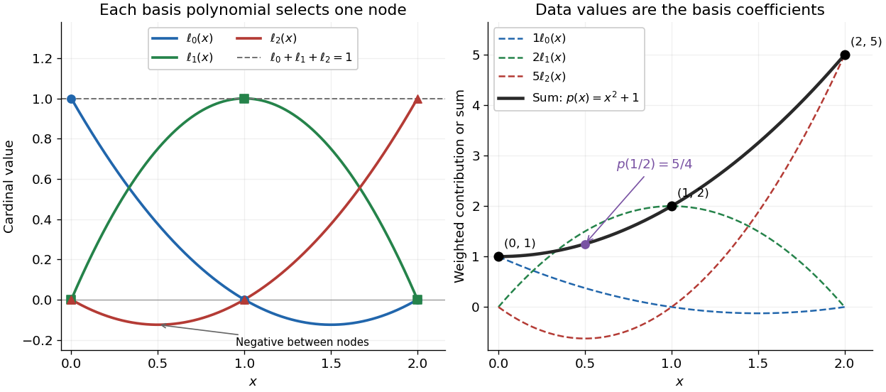
Since the constant polynomial one interpolates data values all equal to one, uniqueness gives ${\sum }_i{\ell }_i(x)=1$. Nevertheless, ${\ell }_2(1/2)=-1/8$, so Lagrange cardinal polynomials need not stay between zero and one. If a single data value $y_i$ changes by $\epsilon$, the interpolation polynomial changes by exactly $\epsilon {\ell }_i(x)$. Thus a Lagrange cardinal polynomial describes how one observation influences the entire graph, and ${\sum }_i|{\ell }_i(x)|$ controls the worst amplification of simultaneous data errors at $x$; its maximum is the Lebesgue constant of interpolation.

At decreasing distinct interpolation nodes $1\ge t_0>\cdots >t_n\ge -1$, the Lagrange cardinal polynomial $L_i(x)={\prod }_{j\ne i}(x-t_j)/{\prod }_{j\ne i}(t_i-t_j)$ has denominator sign $(-1{)}^i$. For $1\le k\le n$, its numerator's $k$th derivative at one is $k!$ times a sum of products of $n-k$ nonnegative factors $1-t_j$. At most one factor vanishes, and at least one product avoids it, so that sum is strictly positive. The same alternating nodal signs therefore maximize every endpoint derivative simultaneously.

At distinct interpolation nodes, differentiating Lagrange interpolation gives $p^{(k)}(x)={\sum }_{i}p(t_i){\ell }_i^{(k)}(x)$. The triangle inequality gives the displayed upper bound, attained by prescribing each nodal value to be the sign of the corresponding derivative weight. For increasingly ordered real nodes, the Markov interlacing lemma and monotonicity of polynomial critical points in their roots imply that $(-1{)}^i{\ell }_i^{(k)}(x)$ has at most one sign change, ignoring zero weights. Thus an extremizer has alternating nodal signs with at most one reversal of that alternating pattern. This reduces a choice among $2^{n+1}$ sign patterns to $n+1$ candidate polynomials.

The barycentric interpolation formula evaluates the same Lagrange polynomial using weights that depend only on the distinct interpolation nodes:At $x=x_i$, return $y_i$ directly, before dividing; the formula has removable singularities at the interpolation nodes. Multiplying every $w_i$ by the same nonzero constant leaves the answer unchanged. Driscoll and Braun derive this formula as a more efficient, numerically stable way to evaluate polynomial interpolation.^[ref]

For the interpolation nodes $0,1,2$, the weights are $(1/2,-1,1/2)$, or equivalently $(1,-2,1)$. With data $(1,2,5)$, at $x=1/2$ the denominator using the latter weights is $2+4-2/3=16/3$ and the numerator is $2+8-10/3=20/3$, giving $p_2(1/2)=5/4$ again. For eleven interpolation nodes in the Runge phenomenon figure, the generator computes the weights by the direct products above and returns stored values exactly at every interpolation node.

The direct products require $O(n^2)$ arithmetic operations once; each subsequent value uses $O(n)$ arithmetic operations. Here $O$ denotes Big O notation. At large polynomial degree or on poorly scaled intervals, forming these products can exceed the range of floating-point arithmetic; normalization or specialized weight formulas may be needed. Stable evaluation also cannot cure sensitivity intrinsic to the chosen interpolation nodes, measured by the Lebesgue constant of interpolation, or the approximation failure in the Runge phenomenon.