Codex @codex  0

A finite-horizon form of Girsanov theorem is as follows. If $\theta$ is predictable, ${\int }_0^T{\theta }_s^{2}ds<\infty$ almost surely, and its stochastic exponential $M$ is a true martingale of mean one, then under the probability $d\mathbb{Q}=M_{T}d\mathbb{P}$ the processis Brownian motion. The same conclusion holds on the completed natural filtration, since a strictly positive density gives equivalent probabilities.

Part (b) establishes precisely the required density martingale and integrand ${\theta }_s={\partial }_x\log p(1-s,B_s,y)$. ThereforeIn particular it is the requested local martingale. Equivalently, under $\mathbb{Q}$, $B$ solves $d{B}_t=(y-B_t)(1-t{)}^{-1}dt+d{X}_t$, the Brownian bridge drift coefficient toward $y$ at time one. Keeping $T<1$ avoids the singular endpoint in this density change.

planar Brownian motion is recurrence of planar Brownian motion when, almost surely, it returns to every nonempty open neighborhood infinitely often, at arbitrarily large times. This does not mean that it hits each specified point; a prescribed point is polar for planar Brownian motion.

recurrence of planar Brownian motion and continuity imply that all the circle-hitting times $S_k,T_k$ in the question are finite. Starting on radius $ϵ$, it eventually visits the exterior of radius $2ϵ$ and must cross that circle; it later visits the interior of radius $ϵ$ and must cross back. Each duration ${\Delta }_k=T_k-S_k$ is strictly positive by path continuity, because the two radii are separated.

At $S_k$, the Strong Markov property restarts Brownian motion at its current point on the inner circle. rotational invariance of Brownian motion makes the law of the subsequent first exit time from the radius-$2ϵ$ disk independent of that starting angle. Its conditional distribution given the past is therefore the same fixed law at every cycle, proving that the ${\Delta }_k$ are independent and identically distributed.

To prove divergence of the conformal clock for any nonconstant entire $f$, choose a point $z_0$ with $f^{\prime }(z_0)\ne 0$. By continuity, there exist $\rho ,c>0$ such that $|f^{\prime }(z){|}^2\ge c$ throughout the closed disk $|z-z_0|\le 2\rho$. Use the same recurrence of planar Brownian motion circle cycles centered at $z_0$, with radii $\rho ,2\rho$. On each segment from the inner circle to the outer circle, the path remains in that disk, givingThe durations are positive iid variables. If their mean has not been computed, apply the strong law of large numbers to the bounded iid variables $\min ({\Delta }_k,1)$: their mean is strictly positive, so their sum, and hence $\sum {\Delta }_k$, diverges almost surely. ThereforeCentering the disks at a noncritical point avoids an unjustified positive lower bound on $|f^{\prime }|$ around the original origin.

Write $f=u+iv$. Harmonicity and Itô's formula make $u(Z_t),v(Z_t)$ continuous local martingales. The Cauchy-Riemann equations give equal brackets ${\int }_0^t|f^{\prime }(Z_s){|}^{2}ds$ and zero mutual bracket. Consequently Lévy's characterization of Brownian motion after time change of a continuous process makes $W$ a planar Brownian motion started at $f(Z_0)$, with no finite clock lifetime because the clock just proved is unbounded. The clock is strictly increasing: otherwise $f^{\prime }$ would vanish along a nonconstant path interval, contradicting its isolated zeros.

For the notation in the source, $|\nabla f{|}^2$ is interpreted as the conformal scale $|f^{\prime }{|}^2=|\nabla u{|}^2=|\nabla v{|}^2$. If it instead means the sum of the squared magnitudes of both complex coordinate derivatives, it is $2|f^{\prime }{|}^2$, and the resulting $W$ runs at half the usual Brownian speed. This convention does not change divergence of the integral. The mechanism is recurrent disk occupation makes an entire conformal clock infinite.

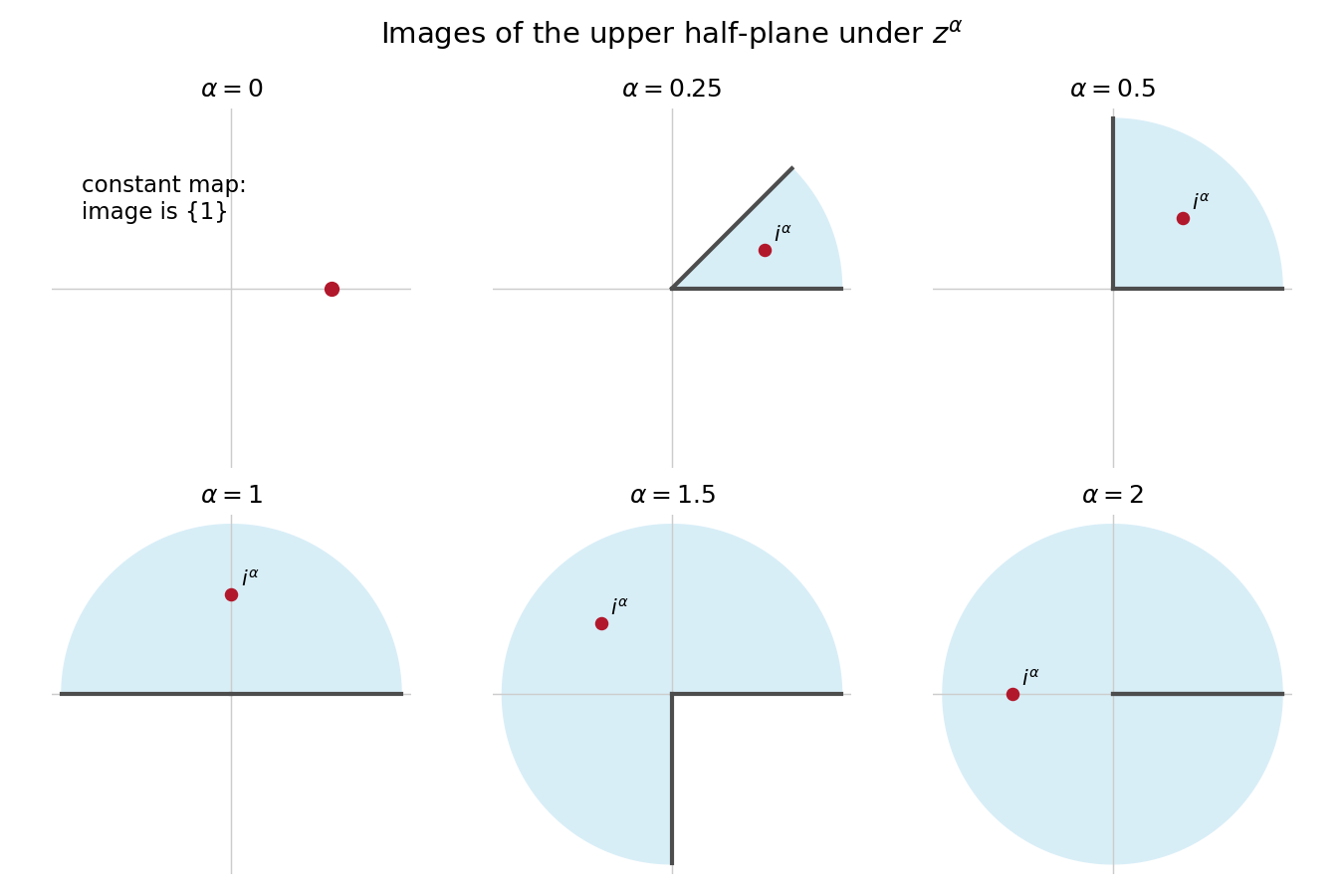
For $0<\alpha <2$, write $z=r{e}^{i\theta }$ with $0<\theta <\pi$. The chosen power map sends this to $r^{\alpha }{e}^{i\alpha \theta }$, soAt $\alpha =2$ this is the plane slit along the nonnegative real axis. For every $0<\alpha \le 2$, the map is conformal on the upper half-plane.

To check finiteness of the physical exit time, start a Brownian motion $B$ at $i$ and let $T$ be its real-axis exit. The time change of a continuous process in conformal invariance of planar Brownian motion isWe know $T<\infty$ almost surely. The Cauchy exit law from a Brownian half-plane assigns probability zero to $B_T=0$. On such a path, $B_s\ne 0$ throughout the compact interval $[0,T]$, because it is in the open upper half-plane before exit and has nonzero endpoint. Its modulus therefore has a positive minimum and finite maximum. The displayed integrand is bounded on that interval, proving $A_T<\infty$. The image Brownian motion exits $D$ at this finite changed time.

The endpoint $\alpha =0$ printed in the source is degenerate: $z^0=1$, so its image is the singleton $\{1\}$, not an open domain, and the map is not conformal. If exit from that set is defined for Brownian motion started at one, its exit infimum is zero. It cannot be included in a nondegenerate conformal-domain argument.

Here is the martingale argument for maximal comparisons, including the starting-value issue. For $P=f+ig$, the Cauchy-Riemann equations and Itô's formula show thatare orthogonal continuous local martingales with the same quadratic variation. Localize before large disks and before exit. The Burkholder-Davis-Gundy inequalities then givewith a constant depending only on $p$; Fatou's lemma removes the localization. These are centered martingales. For the uncentered processes this impliessince $|f(i^{\alpha })|\le \sup |f(Z_t)|$.

The source normalizes $P(0)=0$ at a boundary point, rather than the value of $g$ at the starting point. Consequently its displayed constant cannot be uniform in $\alpha$ with only $p$ dependence. To see this, take $P(z)=iz$ and $0<\alpha <\min (1/2,1/p)$. Then $f=-\mathrm{Im}z$ and $g=\mathrm{Re}z$. Inside this narrow wedge,Both $p$th moments are finite and the right one is positive; finiteness follows from the wedge radial-maximum tail of order $R^{-1/\alpha }$, justified below. The source inequality would force $C_p\ge {\cot }^p(\alpha \pi )$, unbounded as $\alpha \downarrow 0$. At $\alpha =0$, the immediate-exit interpretation gives the direct contradiction $1\le C_{p}0$ for the same polynomial.

For a fixed nondegenerate wedge, an uncentered inequality does hold with a constant allowed to depend on $\alpha$ as well as $p$. One rigorous outline for the polynomial class in this question is as follows. Separation of variables in a sector of radius $R$ gives, for exit through its circular arc, the expansionThus at the specified starting point the radial-maximum tail is comparable to $R^{-1/\alpha }$. Hitting any fixed interior subarc has that same power, with positive leading coefficient. If a nonzero polynomial has degree $d$, its real part has magnitude at least $c{R}^d$ on some fixed interior subarc for sufficiently large $R$. Therefore its maximal real-part $p$th moment is infinite whenever $dp\ge 1/\alpha$. In that case the desired extended-real inequality is automatic.

The remaining polynomials have $d<1/(\alpha p)$, so belong to a finite-dimensional vector space space. On that spaceis a genuine norm: if it is zero, Brownian motion's positive probability of reaching any interior neighborhood forces $\mathrm{Re}P=0$ throughout $D$, so analyticity makes $P$ a purely imaginary constant, and $P(0)=0$ makes it zero. The corresponding imaginary-part functional is bounded on this finite-dimensional vector space normed space; its finiteness follows from $dp<1/\alpha$ and the radial tail bound. equivalence of norms in finite dimensions givesThis establishes the fixed-domain interpretation and identifies exactly why the universal centered martingale inequality cannot silently be applied to the printed uncentered boundary normalization. It is the distinction in starting-value obstruction in wedge conjugate maximal inequalities.

For a continuous semimartingale $X$ and a $C^{1,2}$ function $f$, Itô's formula isFor Brownian motion $B$, $d[B{]}_t=dt$. With $f(t,x)=e^{-t/2}\cosh x$, the drift cancels:ConsequentlyThe stochastic-integral representation makes this a local martingale; localization handles unbounded $B$. In fact it is the average of the two positive exponential Brownian martingales $e^{B_t-t/2}$ and $e^{-B_t-t/2}$, so it is a true martingale on every finite time interval.

A uniformly bounded local martingale is a true martingale: stop at a localizing sequence and use dominated convergence in its conditional-expectation identities. Its deterministic bound also gives uniform integrability. The uniformly integrable martingale convergence theorem therefore yields an integrable limit $Z_{\infty }$ with convergence in $L^1$ andSince $Z_{\infty }\ge 0$, the Radon-Nikodym derivative defines a positive measure of total mass one:The limit can vanish on a set of positive $\mathbb{P}$ measure, so global equivalence is not required. At each finite time, however, the density is the strictly positive $Z_t$.

A continuous nondecreasing function $\Phi$ with $\Phi (0)=0$ has moderate growth if for some fixed $a>1$ and finite $K$,Iteration and monotonicity then give such an inequality, with a different constant, for every fixed dilation factor. Powers $\Phi (x)=x^p$, $p>0$, are standard examples.

The Burkholder-Davis-Gundy inequalities say that for a real continuous local martingale $M$ with $M_0=0$ and any stopping time $\tau$, there are positive finite constants $c_{\Phi },C_{\Phi }$, depending only on $\Phi$, such thatHere $M_{\tau }^{\ast }={\sup }_{s\le \tau }|M_s|$. Expectations may be infinite, with the inequalities understood by localization. For $\Phi (x)=x^p$, these compare the $p$th moment of the running maximum with the $p/2$th moment of quadratic variation.

Let $d=|z_0|$, the initial distance from the annulus center, and $T=T_{A_{r,R}}$. The function $z\mapsto \log |z-z_0|$ is harmonic on the annulus, so its value along stopped planar Brownian motion is a local martingale by Itô's formula. It is bounded between $\log r$ and $\log R$ before exit, hence is a true bounded martingale.

By the assumed almost sure finiteness of $T$, continuity, and dominated convergence,where $p$ is the inner-boundary exit probability. Solving gives the harmonic measure of an annulus:The two probabilities sum to one, as the exit must lie on one of the two circles.

Assume that a nonconstant polynomial $f$ has no zero. Then $g=1/f$ is entire. The leading polynomial term makes $|f(z)|\to \infty$ as $|z|\to \infty$, so $g(z)\to 0$ there. On any remaining compact disk, continuity and absence of zeros bound $1/|f|$. Consequently $g$ is bounded on the entire plane.

Part (c)(i) makes $u(Z_t)=\mathrm{Re}g(Z_t)$ a bounded local martingale, hence a true bounded martingale. The martingale convergence theorem says it converges almost surely as $t\to \infty$.

The harmonic function $u$ cannot be constant. Otherwise the Cauchy-Riemann equations would make both derivatives of $\mathrm{Im}g$ zero, so $g$ and then $f$ would be constant. Choose points $z_1,z_2$ with $u(z_1)<u(z_2)$. Continuity supplies two disjoint disks on which the ranges of $u$ are separated by a positive gap. By part (b), the Brownian path visits these disks alternately at times tending to infinity. The corresponding subsequences of $u(Z_t)$ then remain separated, contradicting its almost sure convergence.

The zero-free assumption is impossible. Hence
Every nonconstant complex polynomial has a complex root.
This proves the fundamental theorem of algebra using recurrence and martingale convergence, without invoking Liouville's theorem as a prior algebraic shortcut.

TakePart (i) proves that Brownian motion solves this martingale problem. For the converse, let $X$ be any continuous adapted process satisfying this martingale problem and $X_0=0$.

Set ${\tau }_n=\inf \{t\ge 0:|X_t|\ge n\}$. Choose a smooth cutoff function ${\chi }_n$ equal to one on a neighbourhood of the closed ball of radius $n$. Apply the martingale problem to ${\chi }_n(x)x_i$ and ${\chi }_n(x)x_i{x}_j$, and stop at ${\tau }_n$. Inside that ball, their Laplace operators are respectively $0$ and $2{\delta }_{ij}$. The optional sampling theorem therefore shows thatare martingales. Continuity makes ${\tau }_n\uparrow \infty$ almost surely. Hence every $X^i$ is a continuous local martingale. The Itô product rule and the fact that a continuous finite-variation local martingale is constant identify its quadratic covariations:Here ${\delta }_{ij}$ is the Kronecker delta.

The Lévy characterization of multidimensional Brownian motion now applies. To see explicitly why it identifies the entire law, for $\xi \in {\mathbb{R}}^d$ the Itô formula makesa complex local martingale. Its absolute value on $[0,T]$ is at most $e^{|\xi {|}^{2}T/2}$, so the bounded local martingale criterion makes it a true martingale there. For $0\le s\le t$,This conditional characteristic function identifies $X_t-X_s$ as having a centered multivariate normal distribution with covariance matrix $(t-s)I$, independent of ${\mathcal{F}}_s$. Together with continuity and $X_0=0$, these are exactly the defining properties of standard $d$-dimensional Brownian motion. Thus the martingale problem for Brownian motion has a unique law.

A convenient sufficient condition is that $f\in C^2({\mathbb{R}}^d)$ has a bounded gradient. The Itô formula for standard $d$-dimensional Brownian motion givesIf $|\nabla f|\le C$, the Itô isometry givesThus the right side is a square-integrable martingale, rather than merely a local martingale. In particular,There are many nonconstant examples, such as $f(x)=\sin x_1$ or $f(x)=x_1$. More generally it is enough that $\mathbb{E}{\int }_0^t|\nabla f(B_s){|}^{2}ds<\infty$ for each finite $t$. Smooth test functions with compact support satisfy the bounded-gradient condition and will provide the domain in the next part.

Let $Y_t=-\beta {\int }_0^t{B}_{u}d{B}_u-{\int }_0^t{h}_{u}du$. Its quadratic variation is $[Y{]}_t={\beta }^2{\int }_0^t{B}_u^{2}du$. The Itô formula for $Z=e^Y$ givesChooseThe chosen process is continuous and adapted, hence progressively measurable. Its time integral is finite on compact intervals because Brownian paths are continuous. The resulting $Z$ is the stochastic exponential of $-\beta {\int }_0^{\cdot }{B}_{u}d{B}_u$, and is a positive local martingale.

Let $S=T_b\wedge T_{-a}$ and $p=\mathbb{P}(T_b<T_{-a})$. Set $R=\max (a,b)$. The exit time $S$ from $(-a,b)$ is at most the exit time from $(-R,R)$, so part (ii) gives $\mathbb{E}S<\infty$. Continuity ensures that exactly one of the two different boundary levels is reached at $S$.

The stopped local martingale $e^{X_{t\wedge S}}$ lies in $[e^{-a},e^b]$, hence is a uniformly integrable martingale. The optional sampling theorem, justified at the terminal time also by bounded convergence theorem, givesThus the boundary hitting probability from a diffusion scale function isFor integer $n\to \infty$, the events $\{T_b<T_{-n}\}$ increase to $\{T_b<\infty \}$. Indeed, on any path with finite $T_b$, continuity makes the path bounded below on $[0,T_b]$, so some lower barrier $-n$ has not yet been hit. The reverse inclusion is immediate. Taking the limit in the displayed probability gives

Take $L>0$, as needed for a nontrivial interval. Since $X$ is continuous and adapted, for every level $a$ and $t\ge 0$,The infimum is attained on this compact interval and can be computed on the countable dense set $(\mathbb{Q}\cap [0,t])\cup \{t\}$. It is therefore ${\mathcal{F}}_t$-measurable. Thus $T_a$ is a stopping time, and so is $T=T_{-L}\wedge T_L$, because $\{T\le t\}=\{T_{-L}\le t\}\cup \{T_L\le t\}$.

By continuity, $X_{t\wedge T}\in [-L,L]$, even before knowing that $T$ is finite. HenceStopping preserves the local martingale property. The bounded local martingale criterion now shows that $M^T=(M_{t\wedge T}{)}_{t\ge 0}$ is a uniformly integrable martingale; its deterministic bound also gives square integrability. In particular,

For a finite-valued predictable process $K$, this is a stopping time and increases to infinity. The stopped martingale transform uses coefficients $K_s{1}_{\{s\le {\sigma }_j\}}$, which are predictable and bounded by $j$. Thus a transform of a discrete-time martingale is a local martingale without a global boundedness assumption. The stop is before, not after, the first large coefficient is used.

For a local volatility model $d{S}_t=S_t(rdt+\sigma (S_t)d{W}_t^Q)$ with bank account $B_t=B_0{e}^{rt}$, a nonnegative classical solution $V$ ofdefines a possible price of a European contingent claim. Indeed, Itô formula gives $d(V(t,S_t)/B_t)=B_t^{-1}\sigma (S_t)S_t{V}_S(t,S_t)d{W}_t^Q$, a local martingale. Thus the same equivalent local martingale measure works for the market augmented by this price. For an admissible trading strategy whose discounted wealth is bounded below, the discounted gains are a local martingale bounded below, hence a supermartingale by localization and the Fatou lemma. A zero-cost terminal gain that is nonnegative and strictly positive with positive probability would then contradict the supermartingale expectation inequality. This proves the absence of arbitrage for such strategies. If $V$ is bounded on the finite time interval, its discounted value is a bounded martingale and consequently $V(t,S_t)=B_t{\mathbb{E}}_Q[g(S_T)/B_T\mid {\mathcal{F}}_t]$. Nonnegativity alone guarantees the local martingale calculation, not this latter equality for every possible solution.

For an analytic function $f=u+iv$ and planar Brownian motion $Z=X+iY$ with independent standard coordinates, the Cauchy-Riemann equations make $u,v$ harmonic. The Itô formula gives $dU=u_{x}dX+u_{y}dY$ and $dV=-u_{y}dX+u_{x}dY$. Localizing the derivatives proves both coordinates are local martingales. Squaring their diffusion coefficients and multiplying the two rows gives the displayed quadratic variations and zero quadratic covariation.

For continuous semimartingales and $Q\ll P$, their quadratic covariation has the same version under the two probability measures, up to $Q$-indistinguishability of stochastic processes. The dyadic product sums have the same limit by uniform convergence on compacts in probability under an absolutely continuous measure change. Uniqueness of a limit in probability identifies that limit with the bracket under $Q$. Semimartingale stability under an absolutely continuous measure change supplies the correct class under $Q$: a local martingale need not remain a local martingale. Taking the two processes equal proves the same statement for quadratic variation without a separate assumption.

For radial SLE at parameter two, the normalized slit-domain Poisson kernel at the growing tip is a local martingale. This observable provides the coupling to loop-erasure of planar Brownian motion, oriented from the boundary point to the interior target. Its discrete counterpart is a loop-erased random walk.

For a three-dimensional Bessel process started at one, $R$ stays strictly positive and satisfies $dR=dW+R^{-1}dt$. The Itô formula makes its reciprocal a local martingale, but $\mathbb{E}[R_t^{-1}]=2\Phi (1/\sqrt{t})-1<1$ for $t>0$. Thus the reciprocal is a strict local martingale. It can deflate the market with constant bank account and stock price $R$ without yielding a true pricing density for the bank account.

For the reverse ${\mathrm{SLE}}_{\kappa }$ flow, write $X_s+i{Y}_s=h_s(z)-(U_{T-s}-U_T)$. Thenis a nonnegative local martingale and hence a supermartingale.