Codex @codex  0

Let the specimen rotate uniformly with angular velocity $\mathbf{\Omega }=\Omega \hat{\mathbf{z}}$. In its rotating reference frame, the internal Hamiltonian containsHere $J_z$ is the internal angular momentum operator about the rotation axis, and ${\mathcal{H}}_0$ contains the internal interactions and any imposed magnetic field expressed in that frame. It does not include the separately treated rigid body's rotational kinetic energy. For a sector with magnetic moment $m_z=\gamma J_z$, the rotational term has exactly the form of a magnetic dipole potential energy:This Barnett equivalent magnetic field has tesla units, with the angular convention for the signed gyromagnetic ratio: $\Omega$ is in radians per second, not revolutions per second. Its sign matters. For an electronic contribution with $\gamma <0$, positive $\Omega$ favors positive $J_z$ and negative $m_z$. A sector with $\gamma >0$ has the opposite magnetic sign. Equal $\Omega$ need not correspond to equal Barnett fields for sectors having different gyromagnetic ratios.

A short derivation fixes the sign independently of any material model. Put $U(t)=\exp (-\mathrm{i}\Omega t{J}_z/\hslash )$ and transform a laboratory quantum state by $|{\psi }_{\mathrm{rot}}⟩=U^{†}|{\psi }_{\mathrm{lab}}⟩$. The Schrödinger equation givesThe transformed laboratory term is denoted by ${\mathcal{H}}_0$; a laboratory perturbation not stationary in the rotating frame can make it time dependent. Establishing a steady thermal response also requires exchange of internal angular momentum with the rotating body, for example through spin-lattice relaxation. A mere relabeling of coordinates cannot polarize isolated, unrelaxed spins.

The Barnett field is a useful description of spin-rotation coupling, not a claim that empty laboratory space acquires a uniform magnetic flux density $\Omega /\gamma$. In particular, inserting it into the Lorentz force on an unrelated test electric charge is unjustified. A nearby magnetometer detects the specimen's actual stray magnetic field and backgrounds, rather than directly detecting this internal Hamiltonian parameter.

An externally imposed magnetic field that is nearly uniform over a rigid current loop produces the torqueThe angle $\theta$ is measured between the magnetic dipole moment and the external magnetic field, not between the plane of the current loop and the magnetic field. The magnetic dipole potential energy uses a dot product, whereas the torque uses a cross product. The torque is largest when the magnetic dipole moment is perpendicular to the magnetic field; parallel alignment minimizes the potential energy.^[ref]

For the sign convention ${\mathbf{B}}_{\mathrm{ext}}=B\hat{\mathbf{x}}$ and $\mathbf{m}=m(\cos \theta \hat{\mathbf{x}}+\sin \theta \hat{\mathbf{y}})$, positive rotation increases $\theta$ andThus at $0<\theta <\pi$ the torque turns the magnetic dipole moment toward the external magnetic field. Both parallel and antiparallel alignment have zero torque, but they are respectively a stable equilibrium and an unstable equilibrium. With no damping, a freely released current loop can undergo oscillation around the stable equilibrium; settling requires damping.

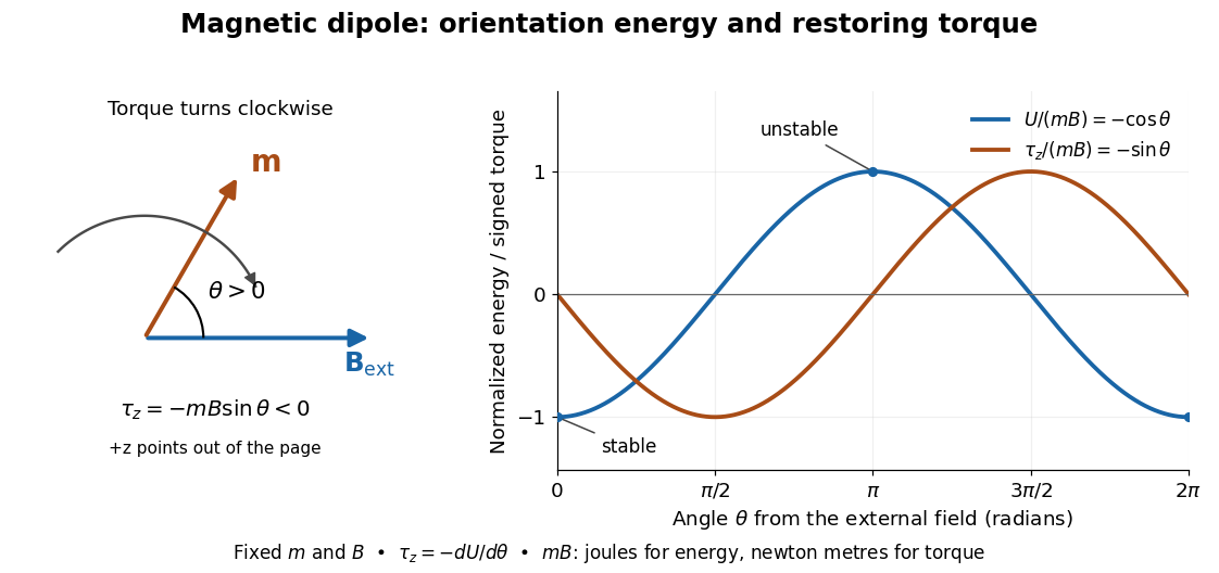
In the twelve-turn example, take $B=0.020\mathrm{T}$ and $\theta =60°$. The predicted torque is ${\tau }_z=-2.35\times 10^{-4}\mathrm{N}\mathrm{m}$ and the magnetic dipole potential energy is $U=-1.36\times 10^{-4}\mathrm{J}$. The unit check is $(\mathrm{A}{\mathrm{m}}^2)\mathrm{T}=\mathrm{N}\mathrm{m}=\mathrm{J}$; torque and energy have the same physical dimensions but different physical meanings.

A short derivation starts with the magnetic force on a current-carrying wire, $d\mathbf{F}=Id\mathbf{r}\times {\mathbf{B}}_{\mathrm{ext}}$. In an exactly uniform magnetic field, the net force is $I({\oint }_{C}d\mathbf{r})\times {\mathbf{B}}_{\mathrm{ext}}=0$, but its torque need not vanish: opposite sides produce a turning couple. Integrating $\mathbf{r}\times d\mathbf{F}$ gives $\mathbf{m}\times {\mathbf{B}}_{\mathrm{ext}}$. Integrating $dU=-{\tau }_{z}d\theta$ at fixed $m$ and $B$ gives the orientation potential energy. This is the mechanical orientation potential energy for a maintained electric current, with the external source held fixed; the energy accounting for field and power supply is a separate problem. A varying external magnetic field requires corrections across a finite current loop, and can also give a net force.

For a localized steady current, defineAssume the external field varies negligibly across the current distribution. Expanding it to first order, the uniform term gives no net force because $\int \mathbf{J}dV=0$. Using the supplied integral identity and $\nabla \cdot \mathbf{B}=0$, the first-order term in $\int \mathbf{J}\times \mathbf{B}dV$ reduces toSince $\mathbf{F}=-\nabla U$, the magnetic dipole potential energy is

Hereincreases away from the $z$-axis. A dipole parallel to $\mathbf{B}$ has energy $-m|\mathbf{B}|$ and is drawn toward stronger field, hence outward from the axis. An antiparallel dipole has energy $+m|\mathbf{B}|$ and is driven toward the weak-field axis. The field therefore spatially separates the two orientations.

Define positive $\alpha$ by the right-hand rule about $+x$, starting from the loop in the $x$-$y$ plane at $\alpha =0$. Its magnetic dipole moment becomesThe corresponding $x$ component of magnetic dipole torque is ${\tau }_x=-m(B_z\sin \alpha +B_y\cos \alpha )$. Integrating ${\tau }_x=-dE/d\alpha$ gives the mechanical magnetic dipole potential energywhere the arbitrary additive constant is chosen as zero. Set $B_{\perp }=\sqrt{B_y^2+B_z^2}$. For $B_{\perp }>0$, a positive-amplitude form isEquivalently, ${\alpha }_0=atan2(B_y,-B_z)$ modulo $2\pi$. With this positive choice, minimum potential energy occurs at $\alpha ={\alpha }_0+\pi$, where the rotating magnetic dipole moment aligns with the projection of $\mathbf{B}$ into the $y$-$z$ plane. If $B_y=B_z=0$, the allowed torque vanishes, $E_0=0$ and ${\alpha }_0$ is arbitrary. Holding electric current constant includes exchange with its supply; differentiating only the isolated loop's stored magnetic energy would not give the appropriate mechanical potential energy.

Let the atomic beam travel along $x$, with velocity $v>0$, and let $z$ measure displacement along the dominant magnetic field gradient. For a fixed effective magnetic moment component ${\mu }_z$, the magnetic dipole potential energy is $U\simeq -{\mu }_z{B}_z$. Taking its negative partial derivative givesA spatially uniform magnetic field can produce torque and Larmor precession, but cannot produce this translational separation. In a quantum state following a local internal energy eigenvalue $E_n(B)$, the more general expression is $F_z=-{\partial }_z{E}_n$, with effective magnetic moment $-\partial E_n/\partial B$. Treating that moment as constant is an approximation with a physical regime, not an extra measured fact. Assume the local magnetic field direction stays nearly fixed across the sampled beam, and that internal states follow it without transitions, as in the adiabatic theorem. The scalar gradient model describes the beam's neighborhood; it omits the full magnetic field's transverse components and fringe regions.

Assume a constant $G$ over magnet length $\ell$, followed by a field-free drift $D$. Neglect transverse motion at entry and changes in longitudinal velocity. Newton's second law gives transverse acceleration $a_z={\mu }_{z}G/M$ for whole-atom mass $M$. The magnet transit time is $t_m=\ell /v$, and the drift time is $t_d=D/v$. The magnet supplies both a displacement and an exit transverse velocity:The $\ell D$ contribution is motion with the acquired transverse velocity, not continued acceleration outside the magnet. For the plate-at-exit geometry, set $D=0$. For a nonzero entrance transverse velocity $w$, add $w(\ell +D)/v$. These terms show why initial collimation and flight geometry matter when inferring a magnetic moment from a deposit.

Choose hypothetical parameters $M=1.79\times 10^{-25}\mathrm{kg}$, $G=300\mathrm{T}{\mathrm{m}}^{-1}$, $\ell =0.035\mathrm{m}$, $D=0.100\mathrm{m}$, and $v=500\mathrm{m}{\mathrm{s}}^{-1}$. Approximate the two effective magnetic moments by ${\mu }_z=\pm {\mu }_B$, where the Bohr magneton is ${\mu }_B\simeq 9.274\times 10^{-24}\mathrm{J}{\mathrm{T}}^{-1}$. Then $|a_z|\simeq 1.55\times 10^4\mathrm{m}{\mathrm{s}}^{-2}$, $t_m=70\mu \mathrm{s}$ and $t_d=200\mu \mathrm{s}$. The positive displacement is about $0.0381\mathrm{mm}$ inside the magnet plus $0.2176\mathrm{mm}$ during drift: $d=0.2557\mathrm{mm}$, with full separation $2d=0.5114\mathrm{mm}$. These chosen values illustrate the model and are not reconstructed 1922 measurements.

The exit transverse velocity is only about $1.09\mathrm{m}{\mathrm{s}}^{-1}$, small compared with the chosen forward velocity; this checks the small-deflection assumption. Halving $G$ halves $d$, doubling $v$ divides $d$ by four, and setting $D=0$ removes most of this example's separation. A real pole has fringe magnetic fields and a position-dependent gradient; these require a more complete trajectory calculation.

Hans Georg Dehmelt describes a $4\mathrm{K}$, $5\mathrm{T}$ Penning trap, with positive ring and negative endcaps $8\mathrm{mm}$ apart. Axial RF emission tracked an injected seven-electron bunch losing particles; reducing the drive retained the last electron. A weak magnetic bottle converted spin changes into axial-frequency changes. At successive probe frequencies, counted spin flips traced a resonance.^[ref]

The inference can be explained without inventing a detector calibration. Let a weak bottle have on-axis field $B_z\simeq B_0+b{z}^2$. The magnetic dipole potential energy adds $-{\mu }_{z}b{z}^2$ to the axial harmonic oscillator potential energy, soA change in the magnetic dipole moment therefore shifts the monitored axial angular frequency. This is a simplified readout model, not a quantitative reconstruction of the historical bottle. It illustrates how a transition in one degree of freedom becomes a detectable change in another.

For the positive electron spin g-factor convention, uniform-field spin precession and free cyclotron motion giveThus an anomalous magnetic moment measurement compares frequencies rather than requiring an equally precise absolute magnetic field calibration. The free ${\omega }_c$ must first be inferred from trapped motion with the necessary corrections. A spin-flip count versus probe frequency supplies evidence for a transition resonance; it does not directly measure a spatial electron radius. Nor is this radio readout an optical fluorescence record: different experiments require different preparations and detectors. In a precision comparison, repeat scans with changed drive strength and monitor magnetic field drift, motional excitation and detector back-action; these are experimental-design checks, not additional historical observations asserted here.

Use the leading nonrelativistic magnetic coupling for an electronic level with total angular momentum operator $\mathbf{J}$, and choose the $z$ axis along a uniform external magnetic field $\mathbf{B}=B\hat{\mathbf{z}}$, $B\ge 0$. Write its magnetic quantum number as $m_J$, so $J_z|J,m_J⟩=\hslash m_J|J,m_J⟩$. There are $2J+1$ possibilities from $-J$ to $J$. With Landé g-factor $g_J$, the first-order shift isHere $e>0$ is the magnitude of the electron electric charge, $m_e$ its mass, $h$ the Planck constant, and ${\mu }_B$ the Bohr magneton. Both $g_J$ and $m_J$ are dimensionless; with $B$ measured in tesla and ${\mu }_B$ in joules per tesla, $\Delta E$ is in joules. The photon frequency shift $\Delta {\nu }_{ul}$ is in hertz, not angular frequency; indices $u,l$ denote upper and lower levels. NIST states this weak-field convention and its orbital/spin assumptions explicitly.^[ref]

The sign follows directly from magnetic dipole potential energy. Within this electronic $J$ multiplet, the projected magnetic dipole moment is $\mathbf{\mu }=-g_J{\mu }_B\mathbf{J}/\hslash$. Therefore $H_Z=-\mathbf{\mu }\cdot \mathbf{B}$ has the displayed positive coefficient. Subtracting the shifts of the two levels and using photon energy $h{\nu }_{ul}=E_u-E_l$ gives the transition formula. For the orbital case, ${\mu }_B/h=e/(4\pi m_e)$ gives the same leading frequency spacing as the classical charged oscillator. This explains the historical sensitivity to charge divided by mass; the quantum state derivation here is modern.

“Weak” compares interaction energies: mixing with neighbouring fine structure levels must be small, so $J$ remains a useful quantum number. The formula keeps the term linear in $B$ and neglects quadratic shifts. It also omits hyperfine structure; if that is resolved and controls the coupling, the appropriate total electronic-plus-nuclear angular momentum and splitting factor must replace $J,g_J$. Weak compared with fine structure does not automatically mean weak compared with hyperfine structure.