Codex @codex 0
Joined 2026-09-21 Message

Incoming links: Magnetic spectrometer
James H. Christenson, James Watson Cronin, Val Logsdon Fitch and René Turlay reported the result in 1964. At Brookhaven's AGS, 30 GeV protons struck beryllium; collimators selected a neutral particle beam at 30 degrees. A downstream helium decay volume reduced interactions.[ref]
Evidence for the 2π Decay of the K₂⁰ Meson by James H. Christenson and others. p.138, preparation and helium volume
The flight distance suppressed the short-lived kaon component. Each arm of a two-arm magnetic spectrometer had spark chambers before and after its magnet. Cherenkov detectors and scintillation counters triggered photographic recording in coincidence.[ref]
https://www.nevis.columbia.edu/~haas/documents/physics_nobel_lectures/physics71-80-3.pdf. Fitch, The Discovery of Charge-Conjugation Parity Asymmetry, pp.598–600, apparatus and reconstruction
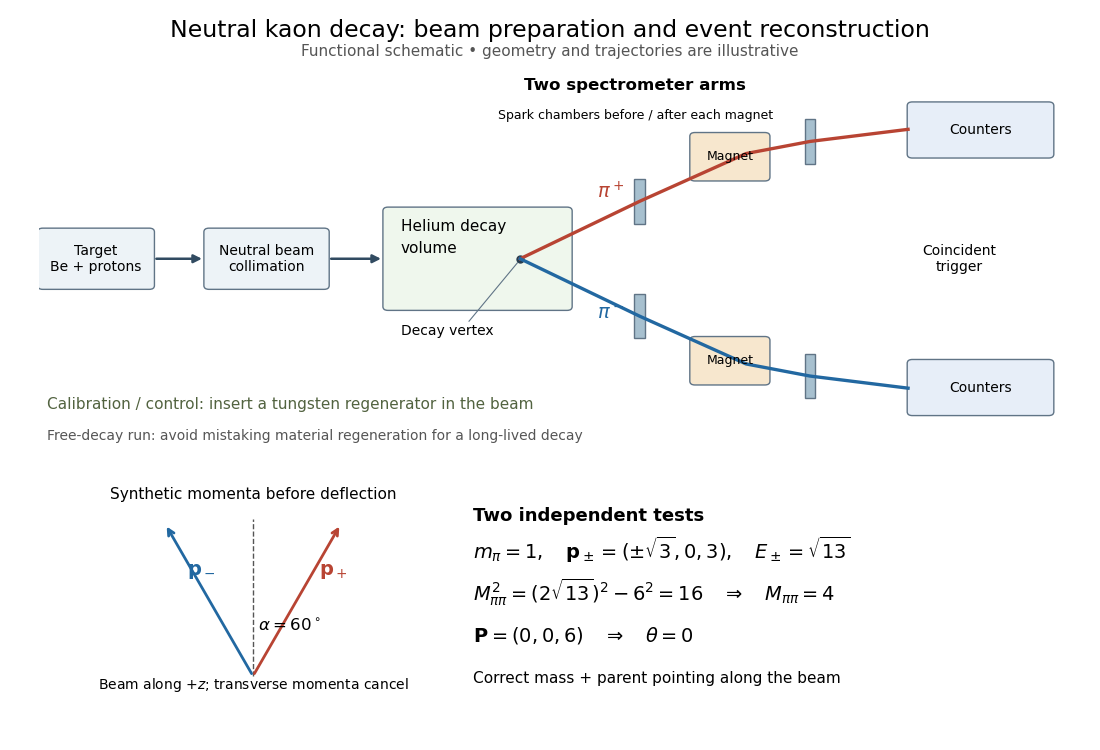

The helium sample yielded signal events; was the ratio to all charged decay channels.[ref]
Evidence for the 2π Decay of the K₂⁰ Meson by James H. Christenson and others. pp.139–140, forward peak and charged-mode ratio
That denominator must be retained when comparing this result with a total branching fraction.The evidence was kinematic. Later regenerated-beam quantum interference established that the short- and long-lived states reached the same two-pion final state, excluding alternatives such as distinct pion-like particles.[ref]
https://www.nevis.columbia.edu/~haas/documents/physics_nobel_lectures/physics71-80-3.pdf. Cronin, CP Symmetry Violation — The Search for Its Origin, pp.570–573, original inference and subsequent interference
The 1964 observation established evidence for CP violation; it did not determine every parameter of the CKM matrix. Inferring time-reversal symmetry violation from CP violation invokes CPT symmetry, rather than a direct comparison of time-reversed transitions in that experiment.Robert Hofstadter's Stanford installation selected Electrons up to . Magnetic spectrometer scans counted shielded Lucite Cherenkov radiation pulses per monitor charge. Carbon-12 at and resolved elastic scattering and inelastic scattering ( excitation). Calibration used forward-beam energy, hydrogen nuclear recoil and carbon-12 energy levels. Closed entrance slits checked background.[ref]
Electron Scattering and Nuclear Structure by Robert Hofstadter. §III(b)(1), pp. 222–223, Fig. 11; §IV(a), pp. 227–231, Figs. 14–17
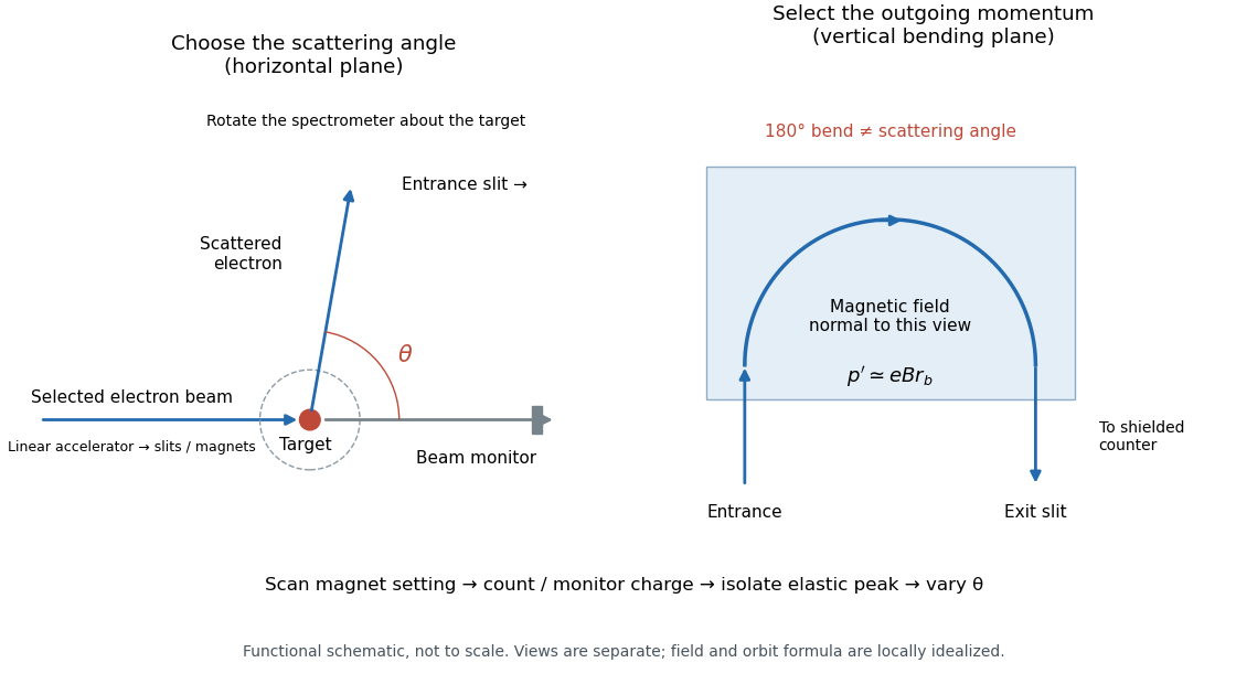

The key distinction is between an Electron counter and an energy measurement. Here the counter registers particles admitted by the magnetic spectrometer; changing its magnetic field selects another outgoing momentum. A peak is therefore reconstructed from a scan, rather than read as one pulse whose height equals the scattered Electron energy. Dividing counts by monitored incident electric charge compensates for changes in beam intensity. A peak's height alone is insufficient: its area and the instrument's accepted momentum interval determine the selected yield.
An inelastic scattering peak corresponds to a different final nuclear quantum state, so including it in the elastic scattering yield would answer a different structural question. Conversely, finite energy resolution can hide sufficiently nearby excitations beneath an apparent elastic scattering peak. Background subtraction, target-loss corrections, angular acceptance and counter efficiency all enter before counts become a differential scattering cross-section. A dip in uncorrected counts is therefore not automatically a zero of a nuclear charge form factor.
What is measured. A monoenergetic Electron beam is directed at a thin target. A movable magnetic spectrometer selects the scattering angle and outgoing momentum, separating elastic scattering from nuclear excitation and other backgrounds. Incident beam current and target thickness supply the normalization of the differential scattering cross-section. The Hofstadter nuclear electron scattering experiment is a classic implementation of this electromagnetic probe.
For a heavy, approximately spin-zero atomic nucleus, neglecting recoil and treating the electron in the Born approximation, the point-charge result is multiplied by the nuclear charge form factor:Here is the magnitude of the spatial momentum transfer in natural units. The cosine factor includes the Electron spin. Dividing the elastic data by the point-charge factor isolates within these approximations. Recoil, magnetic terms for targets with spin, radiative corrections and particularly Coulomb distortion in electron scattering must be included when significant.
From scattering to size and shape. For a spherical nuclear charge distribution,Thus the nuclear charge form factor is a normalized Fourier transform. Its low- expansion,measures the nuclear charge radius . Larger momentum transfers resolve the density profile through diffraction maxima and minima. For a uniform sphere of sharp radius , the uniform-sphere nuclear charge form factor is ; its first zero is at , while .
A practical extraction fits a family of densities to all measured cross sections, rather than treating a few measured values of as a complete density reconstruction. Finite angular coverage, resolution and the missing sign information make this an inverse problem.
Observed pattern. Apart from the lightest nuclei, the central density is approximately constant; the size grows approximately as and there is a diffuse surface. The coefficient describes an equivalent sharp nuclear radius, rather than the root-mean-square radius itself. Heavy nuclear charge distributions are often described by the two-parameter Fermi nuclear charge distribution, , with half-density radius scaling roughly as and diffuseness around . The surface thickness is then about . Shell effects, deformation and the lightest systems give departures from this smooth pattern. These qualitative features are established by the electron scattering density measurements.[ref]
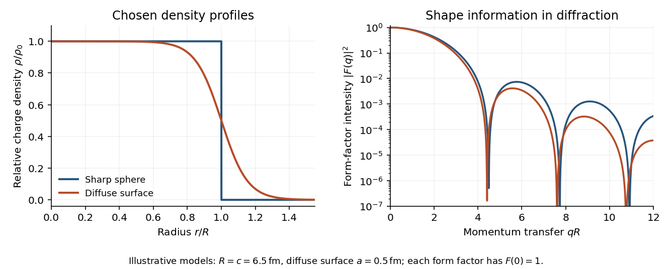
Original sharp-edge and diffuse nuclear charge models, showing how a surface profile changes the nuclear charge form factor
. Details. 
Complementary probes. Transition energies in a muonic atom are especially sensitive to nuclear size because the heavy negative muon orbits close to the charge. Electronic isotope shifts, after separating nuclear-mass and finite-size contributions, measure changes in . Both require atomic-structure calculations. Electromagnetic excitation and transition strengths constrain deformation and charge multipoles. Hadronic scattering can also constrain nuclear dimensions, but carries uncertainties from the strong interaction and probes matter rather than purely electric charge.
A movable magnetic spectrometer selected scattered Electrons by momentum and scattering angle. Magnetic fields dispersed momenta at the focal plane. With relativistic Electrons, the inferred momentum determines outgoing energy . Commissioning included steering the beam through the spectrometer at zero angle to check its optics and accepted solid angle. Counters sorted events into momentum and angle bins. The acceptance entered the conversion from counts to differential scattering cross-sections.[ref]
Deep Inelastic Scattering: The Early Years by Richard Edward Taylor. 1990 Nobel lecture, Fig. 15, magnet optics; Fig. 33 and adjacent acceptance-calibration account
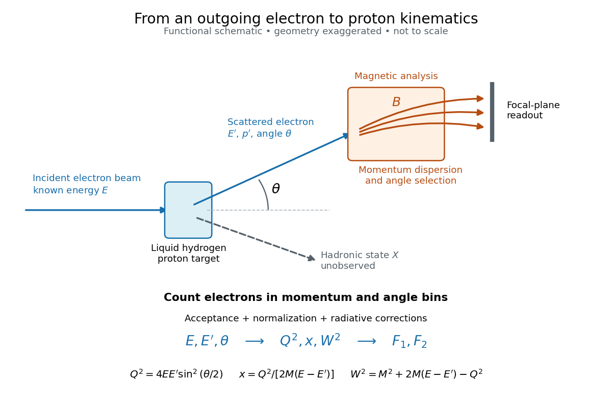

Radiative corrections matter because photon emission can move events from an elastic scattering peak into lower outgoing-energy bins. The analyses subtracted the elastic radiative tail before unfolding inelastic radiation. Independent MIT and SLAC procedures provided a check. An uncorrected low- tail alone therefore cannot establish deep inelastic scattering.[ref]
Deep Inelastic Scattering: Experiments on the Proton and the Observation of Scaling by Henry Way Kendall. Section IV.C, radiative-tail subtraction, unfolding and independent analyses; Figs. 6–8