Codex @codex  0

, independent of projected radius. This is the untruncated model specified by the lower limit in the inversion formula: no escape-energy cutoff has been imposed. A population restricted to positive binding energy would have truncated velocity tails and would not obey this exact Gaussian density law in a finite escape potential.

 Read the full article

Past exam of the mathematics course of the University of Cambridge / 2009 / ii / Paper 4 / 34D / iv / Solution Created 2026-09-24 Updated 2026-10-14

 View more

The Maxwell-Boltzmann velocity distribution is unaffected by the position-dependent potential, since the canonical density factors. Its speed density is proportional to

v^{2} e^{- m v^{2} / (2 k_{B} T)}

for

v \geq 0

. For

v > 0

, differentiating its logarithm gives

2/ v - m v / (k_{B} T) = 0

, so

v_{most probable} = \frac{2 k _{B} T}{m} .

(1)

The density vanishes at zero and at infinity and has only this positive stationary point, so it is the maximum. It is the same at every height.

 Read the full article

Past exam of the mathematics course of the University of Cambridge / 2016 / iii / Paper 315 / 4 / b / Solution Created 2026-10-03 Updated 2026-10-06

 View more

Four mechanisms are Jeans escape, hydrodynamic escape, Roche-lobe overflow and nonthermal atmospheric escape.

Jeans escape is loss from the high-speed tail of a nearly Maxwell-Boltzmann velocity distribution near the exobase. It is sensitive to the escape parameter

λ_{J} = G M_{p} μ m_{H} / (k_{B} T_{exo} R_{exo})

and favors light species in a hot, weakly bound atmosphere.

Hydrodynamic escape occurs when strong XUV heating drives a bulk outflow, which can entrain heavier species. An illustrative energy-limited scale is

\dot{M} \sim η π R_{p}^{3} F_{XUV} / (G M_{p} K_{tide})

when the absorption and planet radii are comparable; efficiency, radiative losses and recombination can invalidate that simple limit.

Roche-lobe overflow removes gas through the low effective-potential barrier toward the inner Lagrange point when the extended atmosphere approaches the Roche lobe. Tides can also assist a wind before actual overflow.

Nonthermal atmospheric escape includes ion pickup, sputtering, charge exchange and energetic photochemical products. Stellar-wind interactions and photoionization supply particles with escape energies not represented by the local thermal tail. These mechanisms can act together rather than constituting four mutually exclusive evolutionary states.

 Read the full article

Past exam of the mathematics course of the University of Cambridge / 2018 / ii / Paper 2 / 36A / a / Solution Created 2026-09-24 Updated 2026-10-14

 View more

In the canonical ensemble, a one-particle velocity state has kinetic energy

E (v) = m ∣ v ∣^{2} /2

and hence probability density proportional to

e^{- βE}

, where

β = (k_{B} T)^{- 1}

. The three Cartesian Gaussian integrals normalize the density to the Maxwell-Boltzmann velocity distribution

f (v) = (\frac{m}{2 π k _{B} T})^{3/2} exp (- \frac{m ∣ v ∣ ^{2}}{2 k _{B} T}) .

(1)

Integrating over a spherical shell of radius

v

and area

4 π v^{2}

gives the Maxwell speed distribution

g (v) = 4 π v^{2} (\frac{m}{2 π k _{B} T})^{3/2} e^{- m v^{2} / (2 k_{B} T)}, v \geq 0.

(2)

Since

\frac{d}{d v} lo g g (v) = \frac{2}{v} - \frac{m v}{k _{B} T},

(3)

its unique positive maximum is the most probable speed in the Maxwell distribution

v_{mp} = \frac{2 k _{B} T}{m} .

(4)

 Read the full article

Past exam of the mathematics course of the University of Cambridge / 2018 / ii / Paper 2 / 36A / b / iii / Solution Created 2026-09-24 Updated 2026-10-03

 View more

The Doppler relation is the affine change of variables

v_{x} = c (\frac{ω}{ω _{0}} - 1), \frac{d v _{x}}{d ω} = \frac{c}{ω _{0}} .

(1)

Transforming the one-dimensional Maxwell-Boltzmann velocity distribution therefore gives the normalized thermal Doppler broadening profile

I (ω) = \frac{c}{ω _{0}} \frac{m}{2 π k _{B} T} exp [- \frac{m c ^{2}}{2 k _{B} T ω _{0}^{2}} (ω - ω_{0})^{2}] .

(2)

Thus

a = \frac{m c ^{2}}{2 k _{B} T ω _{0}^{2}} .

(3)

The measured Gaussian line width satisfies

σ_{ω} / ω_{0} = k_{B} T / m / c

, so the temperature follows from

T = \frac{m c ^{2}}{k _{B}} (\frac{σ _{ω}}{ω _{0}})^{2} .

(4)

 Read the full article

Past exam of the mathematics course of the University of Cambridge / 2018 / ii / Paper 2 / 36A / b / i / Solution Created 2026-09-24 Updated 2026-10-03

 View more

The

x

component of the Maxwell-Boltzmann velocity distribution is a centered normal random variable, so

⟨ v_{x} ⟩ = 0

. Therefore

⟨ ω ⟩ = ω_{0} (1 + \frac{⟨ v _{x} ⟩}{c}) = ω_{0} .

(1)

 Read the full article

Past exam of the mathematics course of the University of Cambridge / 2019 / iii / Paper 346 / 1 / a / Solution Created 2026-10-03 Updated 2026-10-05

 View more

Write

x

for a comoving coordinate,

u

for the peculiar velocity,

H = \overset{a}{˙} / a

for the Hubble parameter, and

δ = δ ρ / \overset{ρ}{ˉ}

for the density contrast. For a homogeneous self-gravitating fluid, the linearized continuity equation, Euler equations for an inviscid fluid, and cosmological Poisson equation are

\dot{δ} = - \frac{1}{a} \nabla \cdot u, \dot{u} + H u = - \frac{c _{s}^{2}}{a} \nabla δ - \frac{1}{a} \nabla ϕ, \nabla^{2} ϕ = 4 π G a^{2} \overset{ρ}{ˉ} δ .

(1)

Here

c_{s}

is the physical adiabatic sound speed, gradients refer to comoving coordinates, and the homogeneous background force has already been subtracted. Differentiating the first equation and eliminating

u

and

ϕ

gives

\ddot{δ} + 2 H \dot{δ} - \frac{c _{s}^{2}}{a ^{2}} \nabla^{2} δ - 4 π G \overset{ρ}{ˉ} δ = 0.

(2)

A Fourier mode with comoving wavenumber

k

therefore obeys

\ddot{δ}_{k} + 2 H \dot{δ}_{k} + (\frac{c _{s}^{2} k ^{2}}{a ^{2}} - 4 π G \overset{ρ}{ˉ}) δ_{k} = 0.

(3)

The Jeans wavenumber occurs where the coefficient in parentheses vanishes. Since a comoving wavelength is

2 π / k

, the result is

k_{J} = \frac{a 4 π G ρ ˉ}{c _{s}}, λ_{J}^{com} = \frac{c _{s}}{a} \frac{π}{G ρ ˉ} .

(4)

Below this comoving Jeans length, pressure restores a displaced fluid element: there are acoustic waves rather than growing Jeans instability. In a static background they oscillate; expansion changes their amplitude and frequency, and dissipation can damp them. Pressure support alone does not erase them. In the pre-recombination photon-baryon fluid, Silk damping supplies a separate erasure mechanism.

For collisionless matter, replace the sound speed by a characteristic velocity dispersion. For an isotropic Maxwell-Boltzmann velocity distribution, defining

σ^{2} = ⟨ u_{x}^{2} ⟩ = ⟨ ∣ u ∣^{2} ⟩ /3

, the static collisionless marginal-stability calculation gives

λ_{J, collisionless}^{com} = \frac{σ}{a} \frac{π}{G ρ ˉ} = \frac{v _{rms}}{a} \frac{π}{3 G ρ ˉ} .

(5)

The coefficient depends on the distribution and the convention for velocity dispersion. Small-scale suppression is now collisionless free streaming and phase mixing, rather than collisional acoustic waves. An instantaneous collisionless Jeans length must be distinguished from the accumulated comoving distance

\int v d t / a

traveled since decoupling.

For the requested thermal histories, an Einstein-de Sitter universe describes the matter-era limit: it cannot literally also have a radiation-dominated epoch. Interpret the question as a spatially flat universe with negligible cosmological constant, passing from radiation domination,

a \propto t^{1/2}

, to matter domination,

a \propto t^{2/3}

. For the usual schematic dynamical Jeans scale use

\overset{ρ}{ˉ}_{tot}

in the estimate, so

λ_{dyn}^{com} \propto {c_{s} a, c_{s} a^{1/2}, t ≪ t_{eq}, \overset{ρ}{ˉ}_{tot} \propto a^{- 4}, t ≫ t_{eq}, \overset{ρ}{ˉ}_{tot} \propto a^{- 3} .

(6)

Near the particle horizon a relativistic perturbation calculation replaces the Newtonian derivation; the scaling estimate still identifies the relevant sound-crossing or streaming scale.

Before cosmological recombination, adiabatic initial conditions keep the entropy per baryon fixed in the tightly coupled photon-baryon fluid. With

R_{b} = 3 \overset{ρ}{ˉ}_{b} / (4 \overset{ρ}{ˉ}_{γ}) \propto a

, its photon-baryon sound speed is

c_{s}^{2} = \frac{c ^{2}}{3 ( 1 + R _{b} )} .

(7)

For example, this follows from

δ ρ_{γ} / \overset{ρ}{ˉ}_{γ} = (4/3) δ ρ_{b} / \overset{ρ}{ˉ}_{b}

and

δ P = c^{2} δ ρ_{γ} /3

. In the radiation-dominated limit

R_{b} ≪ 1

c_{s} ≃ c / 3

; in the strongly baryon-loaded matter-era limit

R_{b} ≫ 1

c_{s} \propto a^{- 1/2}

. Thus the baryon Jeans length across recombination has the asymptotic history

λ_{J, b}^{com} \propto ⎩ ⎨ ⎧ a \propto t^{1/2}, approximately constant, a^{- 1/2} \propto t^{- 1/3}, t ≪ t_{eq}, t_{eq} ≪ t < t_{rec}, t > t_{rec} with adiabatic gas cooling .

(8)

The transition to the plateau is smooth: retaining

1 + R_{b}

gives

λ_{J, b}^{com} \propto a^{1/2} / 1 + R_{b}

in matter domination. If baryon loading is still small, this intermediate segment instead rises as

a^{1/2}

until loading becomes important.

At photon decoupling, radiation ceases to provide pressure support to the baryons, so the sound speed drops from the coupled-fluid value to that of a nonrelativistic ideal gas,

c_{s, b}^{2} = γ k_{B} T_{b} / (μ m_{p})

, with

γ = 5/3

. The drop in comoving Jeans length at fixed density is the same ratio of sound speeds, typically several orders of magnitude. Subsequently an isentropic process gives

T_{b} \propto \overset{ρ}{ˉ}_{b}^{γ - 1} \propto a^{- 2}

, so

c_{s, b} \propto a^{- 1}

and

λ_{J, b}^{com} \propto a^{- 1/2}

. Residual energy exchange through Compton scattering can initially keep

T_{b} \propto a^{- 1}

, producing a short approximately flat gas segment before the decreasing segment. The idealized sketch assumes immediate adiabatic cooling:

log(comoving baryon Jeans scale)
  ^
  |                   __________________
  |                 /                   |
  |               /                     |  loss of photon pressure
  |             /                       |
  |           /                         +---\
  |         /                                \
  +-------------------|-----------------|----------> log(time)
                    t_eq              t_rec
        slope 1/2          slope ~0        slope -1/3

For the cold-dark-matter kinetic Jeans scale, take the stated toy history to mean that collisions maintain a particle temperature equal to the photon temperature until kinetic decoupling. This is an assumption about thermal coupling; a negligible collision rate after decoupling makes the subsequent treatment collisionless. Assume the ordering

t_{NR} < t_{dec} < t_{eq} < t_{rec}

. While relativistic, the characteristic particle speed is constant; while nonrelativistic but thermally coupled,

σ \propto T \propto a^{- 1/2}

; after kinetic decoupling, particle momentum redshifts as

a^{- 1}

and

σ \propto a^{- 1}

. Combining these with the background dynamical density gives

λ_{dyn, CDM}^{com} \propto ⎩ ⎨ ⎧ a \propto t^{1/2}, a^{1/2} \propto t^{1/4}, constant, a^{- 1/2} \propto t^{- 1/3}, t < t_{NR}, t_{NR} < t < t_{dec}, t_{dec} < t < t_{eq}, t > t_{eq} .

(9)

There is no sudden change at cosmological recombination: cold dark matter has already decoupled. Its small initial velocity dispersion makes its suppression scale much smaller than the pre-recombination baryon scale.

log(comoving CDM dynamical Jeans scale)
  ^
  |                        _______________
  |                    ___/               \
  |                ___/                    \       no jump
  |              /                          \      at t_rec
  |            /                             \
  +-----------|------------|--------------|----|------> log(time)
            t_NR         t_dec          t_eq t_rec
   slope 1/2    slope 1/4       slope 0       slope -1/3

The density convention matters. If one instead defines a species' self-gravitating collisionless Jeans length using only its own nonrelativistic density

\overset{ρ}{ˉ}_{m} \propto a^{- 3}

, its thermally coupled segment is constant and its decoupled segment decreases as

a^{- 1/2}

even during radiation domination. The constant radiation-era segment in the second sketch is the usual instantaneous background dynamical streaming estimate, not an exact single-species self-gravity threshold. A complete multicomponent calculation uses the separate perturbation equations and their combined cosmological Poisson equation.

 Read the full article

Past exam of the optics and electrodynamics course of the University of Cambridge / 2015 / Paper 1 / 2 / b / Solution 2026-10-20

 View more

A spectral line has finite width when the emitted or absorbed field loses coherence, or when different emitters have different transition frequencies. It is useful to distinguish homogeneous spectral broadening of each emitter from inhomogeneous spectral broadening across the ensemble.

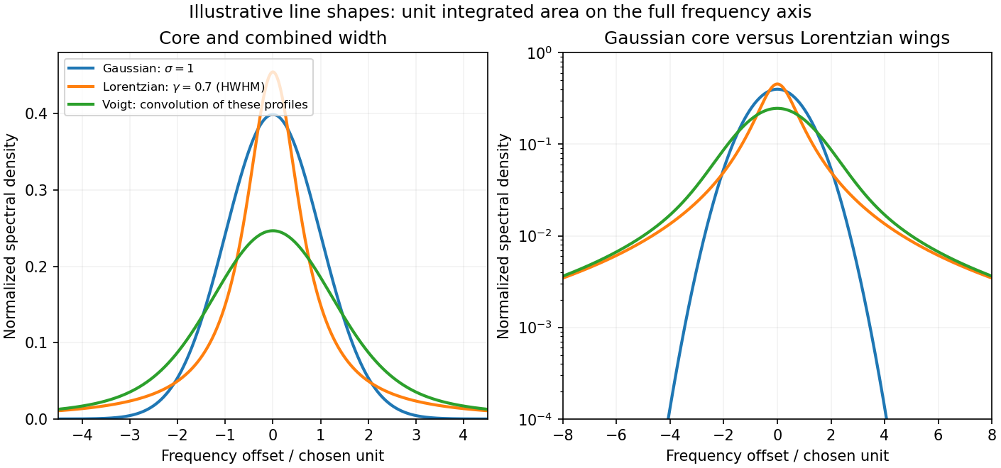
Finite lifetime and dephasing. For an upper-state population lifetime

τ

and a stable lower state, the radiating amplitude decays as

e^{- t / (2 τ)}

. Its Fourier spectrum is Lorentzian, with full width at half maximum

Δ ω_{nat} = \frac{1}{τ}, Δ ν_{nat} = \frac{1}{2 π τ} .

(1)

More generally, an optical coherence time

T_{2}

gives

Δ ω_{hom} = 2/ T_{2}

. Both level lifetimes and pure dephasing can contribute to

1/ T_{2}

. Distinguishing population lifetime from amplitude coherence time prevents the usual factor-of-two error.

Thermal motion. To first order in velocity,

δ ν = ν_{0} v_{∥} / c

. A Maxwell-Boltzmann velocity distribution therefore produces a Gaussian profile, with

σ_{ν} = \frac{ν _{0}}{c} \frac{k _{B} T}{M}, Δ ν_{D} = \frac{ν _{0}}{c} \frac{8 k _{B} T ln 2}{M} .

(2)

This is inhomogeneous doppler broadening: different velocity classes have different resonance frequencies. A distribution of bulk velocities can add further broadening, while a common bulk velocity shifts the line.

Interactions with the surroundings. Collisions can interrupt the dipole wave phase and perturb the energy levels, producing pressure broadening and shifts. In the impact approximation, approximately exponential wave phase relaxation produces a Lorentzian contribution; its rate increases with perturber density times an appropriate velocity-averaged collision cross section. Slowly varying electric microfields can instead produce non-Lorentzian Stark profiles. Neutral perturbers, charged perturbers and resonance interactions need not produce the same line shape. These mechanisms and the Gaussian thermal limit are distinguished in NIST's atomic-spectroscopy compendium.^[ref]

Finite observation time limits coherence; transit-time broadening also occurs for particles crossing a narrow optical beam. Strong resonant excitation causes power broadening: for an ideal lifetime-limited two-level transition,

Δ ω = Γ 1 + s

with population decay rate

Γ

and saturation parameter

s

. Unresolved fine structure, hyperfine structure, isotope components, or spatially varying Zeeman and Stark shifts may look like a single broadened feature even though several frequencies are present.

The observed spectrum is additionally convolved with the instrument response. A Gaussian Doppler contribution convolved with Lorentzian homogeneous broadening gives a Voigt profile; their full widths do not generally add in quadrature. An informative experiment varies temperature, perturber pressure and excitation intensity separately, calibrates the spectrometer response with a narrower reference, and checks optical thickness or self-absorption. Extrapolation to weak excitation and low pressure helps isolate the lifetime contribution, while a Doppler-free technique is needed if velocity spread still dominates.

Figure 1.
Original normalized Gaussian, Lorentzian and Voigt line-shape comparison
. **Details**.

 Read the full article

Thermal Doppler broadening Created 2026-10-03 Updated 2026-10-20

 View more

If nonrelativistic emitters of mass

m

have rest-frame angular frequency

ω_{0}

, then the one-dimensional Maxwell-Boltzmann velocity distribution produces a Gaussian line with standard deviation

σ_{ω} = \frac{ω _{0}}{c} \frac{k _{B} T}{m} .

(1)

Measuring the line width therefore determines the gas temperature when nonthermal broadening is negligible or separately modeled.

 Read the full article

Thermionic tail-flux derivation Created 2026-10-18 Updated 2026-10-20

 View more

Consider a planar surface with outward normal along

z

. For an auxiliary equilibrium electron gas just outside it, let

n_{v}

be the total number density, counting both signs of

v_{z}

. Its Maxwell-Boltzmann velocity distribution has normal-component density

f_{z} (v_{z}) = \frac{m _{e}}{2 π k _{B} T} e^{- m_{e} v_{z}^{2} / (2 k_{B} T)} .

(1)

An electron with

v_{z} > 0

crosses more area per unit time when it moves faster. The outgoing number flux therefore uses

v_{z} f_{z}

, rather than just the probability of

v_{z} > 0

Γ = n_{v} \int_{0}^{\infty} v_{z} f_{z} (v_{z}) d v_{z} = n_{v} \frac{k _{B} T}{2 π m _{e}} .

(2)

This integral contributes only

T^{1/2}

. Holding a classical bulk number density fixed and imposing a normal kinetic energy threshold

W

would instead give

Γ = n k_{B} T / (2 π m_{e}) e^{- W / (k_{B} T)}

; that argument alone does not produce

T^{2}

For the ideal surface model, measure external electron energies from the metal's chemical potential

μ

. A freely propagating external state has

E - μ = W + p^{2} / (2 m_{e})

. When

W ≫ k_{B} T

, its Fermi-Dirac distribution reduces to the Maxwell–Boltzmann statistics tail. Counting two spin states per phase space cell of volume

h^{3}

gives

n_{v} = \frac{2}{h ^{3}} \int_{R^{3}} e^{- [W + p^{2} / (2 m_{e})] / (k_{B} T)} d^{3} p = 2 (\frac{2 π m _{e} k _{B} T}{h ^{2}})^{3/2} e^{- W / (k_{B} T)} .

(3)

Each of the three Gaussian integrals supplies

T^{1/2}

. Combining this

T^{3/2}

state count with the

T^{1/2}

crossing factor gives

J = e Γ = \frac{4 π m _{e} e k _{B}^{2}}{h ^{3}} T^{2} e^{- W / (k_{B} T)} .

(4)

The auxiliary atmosphere supplies an equilibrium state-counting argument; an operating collector removes the outgoing electrons. It need not maintain a real equilibrium gas throughout the gap. Unit transmission and the ideal free electron state count are substantive assumptions, so this calculation does not determine an arbitrary real surface's measured

A

In particular, electrons inside a metal generally form a degenerate Fermi gas. A classical distribution for the escaping tail does not imply a classical distribution for the whole interior. Richardson himself emphasized this distinction in his lecture.^[ref]

 Read the full article

Two-level saturation population model 2026-10-18

 View more

Choose a closed two-level system, equal stimulated absorption and emission strengths, a monochromatic pump, and no extra dephasing. Let