Baryon

A baryon is a hadron with half-integer spin and baryon number one; ordinary baryons consist of three valence quarks.

A baryon containing one or more strange quarks and no heavier quark. The light hyperon multiplets include lambda, sigma, xi and omega baryons. Strong and electromagnetic interactions conserve strangeness, whereas a weak interaction can change it; a photon in the final state does not by itself make a hyperon decay electromagnetic.

A strong interaction decay must conserve quark flavour and have final rest energy below the initial mass. An excited light baryon can often decay to a lighter baryon plus a pion. A ground-state strange baryon may lack any such open flavour-conserving channel even when its spin permits one. In particular, the Omega baryon cannot decay strongly to a Xi baryon plus a pion because that changes strangeness; its flavour-conserving Xi-kaon channel is closed by the mass threshold. A spin-three-half assignment alone does not imply a strong decay.

An antibaryon is the antiparticle of a baryon. In the valence quark model it consists of three antiquarks in a colour singlet. Charge conjugation reverses its additive charges and third component of isospin, preserving total isospin and spin.

A baryon containing a charm quark. For one charm and two up/down quarks in the spatial ground state, light-diquark spin-isospin correlation gives the isosinglet Lambda c baryon and the isotriplet Sigma c baryon families.

The symmetric light pairs $uu,\{ud\},dd$ with one charm quark give isospin one and charges $2,1,0$. Their light spin is one; coupling the charm spin gives the $J=1/2$ Sigma c baryon triplet and $J=3/2$ excited-spin triplet conventionally marked by a star.

The lowest Lambda c baryon has valence content $cud$, electric charge $+1$, isospin zero and spin angular momentum $1/2$. Its light pair has antisymmetric flavour and spin zero. This is the charm analogue of the Lambda baryon.

The light-quark $sss$ member of the spin-three-halves baryon decuplet has strangeness $S=-3$, baryon number $B=1$, flavor hypercharge $Y=-2$, and isospin zero. The Gell-Mann--Nishijima formula gives electric charge minus one. Its position at the bottom of the decuplet's triangular weight diagram follows by replacing all three up or down quarks with strange quarks.

The 1964 report exposed Brookhaven's 80-inch hydrogen bubble chamber to a mass-separated $5.0\mathrm{GeV}/c$ negative-kaon beam. A photographed decay chain, track momenta and bubble density supported the particle identification. Two converted photons helped reconstruct a neutral pion. Alternative assignments were tested kinematically. The authors reported an Omega baryon candidate with $Q=-1$, $S=-3$ and mass $1686\pm 12\mathrm{MeV}/c^2$, reserving a detailed systematic-error discussion for further events.^[ref]

This is an inference from several linked observations. A charged particle can leave a visible bubble-chamber track, while a neutral segment must be reconstructed from its production and decay products. Agreement between possible decay channels, electric charge, momentum conservation and the reconstructed mass is stronger evidence than a suggestive track shape alone. The event tests a predicted hadron pattern; it does not photograph the three strange quarks individually.

For example, an independently constructed two-body kinematic check usesIn a parent rest frame with equal and opposite daughter momenta, the momentum sum vanishes, giving $M{c}^2=E_1+E_2$. In units $c=1$, stipulated daughter masses $m_1=1$, $m_2=1/4$ and momentum magnitude $p=3/4$ give $E_1=5/4$, $E_2=\sqrt{10}/4$ and $M=(5+\sqrt{10})/4\simeq 2.04057$. A common Lorentz boost changes the daughter energies and momenta while preserving this reconstructed invariant mass. These chosen units and numbers are an illustration, not a reanalysis of the 1964 event.

A baryon with constituent content four quarks and one antiquark, whose net baryon number is one. Such content admits more flavour representations than three quarks alone. A representation in the tensor product is not evidence by itself of a bound state.

Exotic flavour weights can decay into a baryon and a meson while preserving every strong quantum number: $uudd\bar{s}\to p{K}^0$ or $n{K}^{+}$, $ddss\bar{u}\to {\Xi }^{-}{\pi }^{-}$, and $uuss\bar{d}\to {\Xi }^0{\pi }^{+}$. These are quark rearrangements. If above threshold with unsuppressed couplings, such states are short-lived strong resonances. Flavour symmetry alone fixes neither masses nor widths.

Two antisymmetric flavour quark pairs can each transform in $\overline{3}$, combine into $\overline{6}$, and with an antiquark give $\overline{6}\otimes \overline{3}=\overline{10}\oplus 8$. The antidecuplet rows are $(Y,I)=(2,0),(1,1/2),(0,1),(-1,3/2)$. Exactly three weights are absent from all three-quark states: $(I_3,Y)=(0,2)$ and $(\pm 3/2,-1)$.

In a three-quark colour singlet, a symmetric spatial state requires symmetric spin-flavour symmetry. Completely symmetric decuplet flavour couples to symmetric spin $3/2$; mixed octet flavour couples to mixed spin $1/2$ in the symmetric permutation combination. Antisymmetric singlet flavour cannot have a symmetric S-wave orbital state, since ${\bigwedge }^3{\mathbb{C}}^2=0$ forbids a completely antisymmetric state of three spin-$1/2$ quarks. Mixed orbital and spin states can instead realize the required antisymmetry.

Two light quarks in a symmetric spatial state and the antisymmetric colour pair inside a three-quark colour singlet require symmetric spin-flavour symmetry. Their isospin singlet and spin singlet are both antisymmetric, while their respective triplets are symmetric. Thus the allowed pairs have $(I,S_{ud})=(0,0)$ or $(1,1)$; opposite exchange parities are excluded. Coupling an isospin-zero spin-one-half quark gives an $I=0,J=1/2$ baryon or $I=1,J=1/2,3/2$ baryons.

For an isospin singlet quark $h$ of charge $q_h$, the antisymmetric light-flavour pair gives an $I=0,J=1/2$ state with charge $q_h+1/3$. The symmetric light-flavour pairs $uu,\{ud\},dd$ give $I=1$ triplets of spins $1/2$ and $3/2$, with charges $q_h+4/3,q_h+1/3,q_h-2/3$. These follow from light-diquark spin-isospin correlation and addition of constituent electric charges, with zero orbital angular momentum.

Three light quarks have a six-dimensional single-quark spin-flavour space ${\mathbb{C}}^3\otimes {\mathbb{C}}^2$. A symmetric spatial ground state and the antisymmetric three-quark colour singlet require the symmetric cube of that space. Its dimension is $\left(\genfrac{}{}{0ex}{}{8}{3}\right)=56$, and restriction to flavour $SU(3)$ and spin $SU(2)$ gives a baryon decuplet of spin $3/2$ and a baryon octet of spin $1/2$. The two mixed-permutation multiplicity spaces pair once in the symmetric sector, explaining why the two flavour-octet copies in the unconstrained tensor cube do not represent two distinct ground-state octets.

The invariant colour state of three fundamental quarks is the normalized completely antisymmetric tensor ${ϵ}_{abc}/\sqrt{6}$. With this colour factor, the Pauli exclusion principle requires the remaining spatial-spin-flavour wavefunction to be symmetric. Colour and approximate flavour symmetry are distinct SU(3) actions.

If three quarks are hypothetically spin-zero bosons, their total state is symmetric under particle exchange. In an $L=0$ symmetric spatial state, the unchanged antisymmetric three-quark colour singlet therefore requires an antisymmetric quark flavour state. With three flavours its space is ${\bigwedge }^3{\mathbb{C}}^3$, of dimension one. The sole flavour state contains one quark of each flavour and has total angular momentum zero.

For an identical-flavour pair in the symmetric spatial ground state of a baryon, the flavour factor is symmetric and the three-quark colour singlet is antisymmetric under their exchange. The Pauli exclusion principle therefore requires a symmetric pair spin factor. Two spin-one-half quarks then form a triplet state, $S_{qq}=1$, rather than a spin singlet. The conclusion applies to the identical pair in both spin-one-half and spin-three-half ground-state baryons.

The baryon octet contains the isospin doublet ${\Xi }^0,{\Xi }^{-}$. Each has strangeness $-2$, with valence quark content $uss$, $dss$.

The baryon octet contains an isospin triplet ${\Sigma }^{+},{\Sigma }^0,{\Sigma }^{-}$. Each has strangeness $-1$; their valence quark contents are $uus$, $uds$, $dds$.

The neutral Sigma baryon and Lambda baryon both have valence content $uds$, but different spin-isospin couplings. An electromagnetic transition changes those internal couplings without changing any quark flavour. In the simple ground-state quark model, the nonzero magnetic transition is associated with the up- and down-quark electromagnetic currents; the strange-quark spin operator alone cannot change the $ud$ pair from spin one to spin zero. Four-momentum conservation gives photon energy $E_{\gamma }=(M_{\Sigma }^2-M_{\Lambda }^2)/(2M_{\Sigma })$ in natural units.

The ${\Lambda }^0$ in the baryon octet is an isospin singlet with strangeness $-1$ and zero electric charge. Its ordinary valence quark content is $uds$.

The proton and neutron form the nucleon isospin doublet, with spin angular momentum $1/2$ and baryon number one. A unit Skyrmion with the fermionic Finkelstein-Rubinstein constraints gives these quantum numbers in its lowest rotational multiplet.

The proton is the positively charged spin-one-half baryon found in atomic nuclei. Its mass is approximately $1836$ times the electron mass.

The root mean square radius of the proton charge distribution. Finite nuclear size changes hydrogen atom energy levels and enters precision predictions for the Lamb shift.^[ref]

The neutron is the electrically neutral spin-one-half baryon found with protons in most atomic nuclei.

A neutron is a nucleon: it contributes to an atomic nucleus without adding electric charge. Its spin one-half makes it a fermion, and it belongs to the baryons. Electrical neutrality does not mean an absence of interactions: a neutron can transfer momentum and kinetic energy to an atomic nucleus, producing a charged nuclear recoil that a particle detector can register. This indirect route is central to neutron detection by proton recoil.

The beautiful feature of the Chadwick neutron discovery experiment is that an unseen projectile acquired a measurable mass through the motion of things it struck. Penetration alone left competing explanations open; combining nuclear recoils from different target masses supplied a much stronger test.

A neutron released on the short timescale associated with the fission event, rather than after a precursor radioactive transformation. Prompt describes emission timing, rather than the neutron speed after subsequent scattering.

A neutron emitted following a radioactive transformation of a precursor, rather than promptly in the original nuclear fission. The waiting time reflects the precursor lifetime. It is distinct from the later detection of a prompt neutron after scattering or moderation.

The fraction of fission-related neutron production assigned to delayed neutrons under the chosen averaging convention. Effective kinetics parameters can include spatial and spectral weighting; a small fraction can still have a large influence on population timescales.

A radioactive fission product whose decay chain can populate a neutron-emitting daughter state. A simplified kinetics model can replace many such species by one effective population and lifetime, losing the distinct decay-time spectrum.

Neutron scattering measures how a specimen changes the directions and kinetic energies of incident neutrons. Neutron diffraction uses the elastic scattering pattern to investigate crystal structure and magnetic order; inelastic neutron scattering uses energy transfer to investigate excitations such as phonons and magnons. The two measurements ask complementary questions: what arrangement repeats in space, and what disturbances can propagate through it?

The 1994 Nobel Prize in Physics recognized Clifford Glenwood Shull's diffraction work and Bertram Neville Brockhouse's spectroscopy.^[ref]

Nuclear scattering couples to atomic nuclei; magnetic scattering couples the neutron's magnetic moment to electronic magnetic moments. The latter underlies both magnetic neutron diffraction and magnon spectroscopy. An atomic number is not a nuclear neutron scattering weight: the relevant coefficient in the elementary coherent model is the nuclear neutron scattering length.

A neutron-scattering technique using small momentum transfer to probe larger-scale structure. Contrast, background subtraction and the measured wave-number range determine which structural parameters can be inferred.

Thickness-dependent interference oscillation from reflections at the two sides of a film. At sufficiently large normal momentum transfer, the fringe spacing is approximately $2\pi /d$.

The sum of nuclear coherent scattering lengths per unit volume, ${\rho }_b={\sum }_j{n}_j{b}_j$. Matching it between media suppresses their ideal interface contrast.

Treat the incident and outgoing neutrons as free nonrelativistic particles outside the specimen. Their wave vectors, de Broglie wavelengths, momenta and kinetic energies obeyHere $k_i=|{\mathbf{k}}_i|$, $k_f=|{\mathbf{k}}_f|$, $m_n$ is the neutron mass, and $\hslash =h/(2\pi )$ uses the Planck constant. Subtracting the outgoing projectile quantities from the incoming ones gives the momentum transfer and energy delivered to the specimen:Thus $\mathbf{Q}$ has units of inverse length, rather than momentum. A positive $\omega$ means the specimen gains energy; negative $\omega$ means it supplies energy to the neutron. If the angle between incident and outgoing propagation directions is $2\theta$, the law of cosines givesKnowing the detector angle alone therefore leaves $Q$ undetermined unless the outgoing energy is known or an elastic scattering assumption is justified.

For a reproducible unit conversion choose $m_n=1.67492750056\times 10^{-27}\mathrm{kg}$, $h=6.62607015\times 10^{-34}\mathrm{J}\mathrm{s}$ and $1\mathrm{eV}=1.602176634\times 10^{-19}\mathrm{J}$. The first is a recommended central value; the latter two conversions are exact.^[ref] With $1$ ångström equal to $10^{-10}\mathrm{m}$ and $1\mathrm{meV}=10^{-3}$ electronvolts, substitution into $E=h^2/(2m_n{\lambda }^2)$ givesSquare brackets here mean the numerical value in the indicated unit. For an original chosen example, ${\lambda }_i=2$ ångströms and ${\lambda }_f=2.5$ ångströms give $E_i\simeq 20.451\mathrm{meV}$, $E_f\simeq 13.089\mathrm{meV}$ and $\hslash \omega \simeq 7.362\mathrm{meV}$. At $2\theta =60^{\circ }$, $Q\simeq 2.879{\mathring{\mathrm{A}}}^{-1}$. These values stipulate an allowed projectile geometry; they do not assert that any particular specimen has an excitation there.

Define transfer gained by the neutron as $\mathbf{Q}={\mathbf{k}}_f-{\mathbf{k}}_i$. If it is perpendicular to ${\mathbf{k}}_i$, expansion of the free-neutron kinetic energy gives $E_f-E_i={\hslash }^2{Q}^2/(2m_n)$. Absorbing one phonon requires this positive energy to equal $\hslash \omega$. A periodic phonon branch may therefore intersect a nonperiodic recoil parabola in an extended-zone representation. The sign of $\mathbf{Q}$ is opposite to the common sample-transfer convention and must be declared.

In neutron diffraction, coherent elastic scattering adds scattering amplitudes from regularly positioned scatterers. Since $E_f=E_i$, the neutron scattering kinematics gives $k_f=k_i=2\pi /\lambda$ andFor lattice planes of interplanar spacing $d_{\mathrm{p}}$, constructive addition requires $Q=2\pi n/d_{\mathrm{p}}$ along the plane normal. Equating these expressions proves Bragg's law:For example, stipulate $d_{\mathrm{p}}=2$ ångströms and $\lambda =2$ ångströms. The first diffraction order has $\theta =30^{\circ }$ and detector deflection $60^{\circ }$. A peak position constrains a period; its intensity also depends on the crystal basis structure factor.

Clifford Glenwood Shull describes powdered sodium chloride, a crystal monochromator, and a shielded counter recording angular counts. Inserting cadmium measured background; substantial diffuse scattering complicated peak interpretation.^[ref]

Powdering supplies many crystal orientations. Comparing the angular peaks with Bragg's law constrains crystal structure; a background estimate helps distinguish specimen peaks from unwanted counts. A two-axis diffraction instrument has no separate outgoing energy analysis, so an angular pattern alone does not separate every inelastic contribution. The richer magnetic example, including a warm/cold comparison and its limits, is the manganese monoxide neutron diffraction experiment. Its extra peaks reveal magnetic order beyond the chemical periodicity; the associated magnetic neutron diffraction model is developed there.

The nuclear neutron scattering length is the effective length coefficient for low-energy nuclear scattering amplitude. For the elementary coherent calculation below, use a bound coherent coefficient $b_j$ for each site, and neglect absorption so that $b_j$ is real. This coefficient describes the atomic nucleus, including its isotope and nuclear spin dependence; it is not proportional to atomic number. Replacing nuclear coefficients by electronic magnetic moments would describe a different scattering channel, with additional direction and spatial-distribution factors, as explained in magnetic neutron diffraction.

Choose a one-dimensional crystal with cell translation $a$ and two atoms per cell at $0$ and $d=a/2$. Here $d$ is an intracell displacement, distinct from the interplanar spacing $d_{\mathrm{p}}$ above. In a single-scattering approximation, a row of $N$ cells has scattering amplitudeThe sum selects reciprocal lattice positions $Q_h=2\pi h/a$ as $N$ becomes large. At these positions, the two-site crystal basis structure factor and its squared magnitude areConsequently $b_1=b_2=b$ gives even reflections of strength $4b^2$ and extinguishes the odd reflections. Choosing $b_1=b$, $b_2=b/2$ instead gives $9b^2/4$ and $b^2/4$: the odd/even ratio is $1/9$. Equal atomic numbers would not establish equal $b_j$ if the isotopes differ. The figure below plots these chosen coefficients, without assigning them to actual elements. Missing reflections can encode destructive wave interference within a cell, not the absence of matter at a site.

Inelastic neutron scattering resolves $E_i-E_f\ne 0$. Through conservation of energy, a peak at positive $\hslash \omega$ identifies an allowed excitation energy; through momentum conservation, its location in $\mathbf{Q}$ constrains the spatial variation of that excitation. A phonon is a quantum of lattice vibration; a magnon is a quantum of a spin wave. Their different couplings make energy transfer alone insufficient to identify which was created.

Bertram Neville Brockhouse's aluminium experiment rotated a large single crystal, scanning analyzer angle for neutron groups. His vanadium comparison exposed the elastic resolution. Later magnetite measurements used a magnetic field intensity test to identify magnons.^[ref]

Successive orientations sample different wave vectors; analyzer settings distinguish outgoing energies. This supplies points on a dispersion relation, rather than only an angular diffraction pattern. Finite resolution can merge neighboring excitations; background, multiple scattering and processes involving several phonons can complicate interpretation. A lattice model is a testable explanation of selected features, not a guarantee that every spectral peak has the same origin.

A triple-axis spectrometer uses Bragg's law at an initial crystal monochromator to select ${\lambda }_i$ and at a second analyzing crystal to select ${\lambda }_f$. The sample sits between these selectors. The three axes refer to the monochromator, sample and analyzer rotations. The final counter measures accepted counts; the analyzer's wavelength selection makes those counts sensitive to outgoing energy even when the counter does not measure each neutron's energy directly.

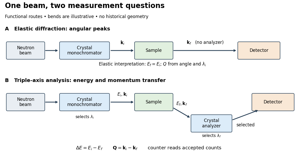
For a constant-$\mathbf{Q}$ scan, change incident or outgoing energy while coordinating sample and analyzer settings so that ${\mathbf{k}}_i-{\mathbf{k}}_f$ stays fixed. Counts versus $E_i-E_f$ then probe excitations at one momentum transfer. Changing only the analyzer angle generally changes both transferred quantities. Incident-beam monitoring, analyzer response and the instrumental resolution must enter quantitative interpretation; the diagram's arrows specify information flow, not an absolute intensity calibration.

Consider an original ideal one-dimensional monatomic harmonic oscillator chain with neighbor separation $a$, mass $M$ and nearest-neighbor restoring coefficient $K>0$. Its displacement equation isSubstitute the normal mode $u_r=u_0{e}^{i(qra-\omega t)}$. Since $e^{iqa}+e^{-iqa}-2=-4{\sin }^2(qa/2)$,Choose $a=4$ ångströms and ${\epsilon }_{\ast }=10\mathrm{meV}$. This is one acoustic phonon branch, distinct from the two-atom elastic example. It has $\epsilon (\pi /(2a))=5\sqrt{2}\mathrm{meV}$ and $\epsilon (\pi /a)=10\mathrm{meV}$.

For coherent creation of one phonon in a crystal, the excitation's wave vector $q$ and the measured transfer obey $Q=G+q$, with $G$ a reciprocal lattice vector. To connect the dispersion relation to an illustrative intensity, take zero temperature, longitudinal displacements and the first interval $Q=q\in (0,\pi /a]$, choosing $G=0$. Expand the scattering phase to first order, $e^{iQ(ra+u_r)}\simeq e^{iQra}(1+iQ{u}_r)$. The constant term supplies elastic scattering; the linear term creates one phonon. Its displacement matrix element is proportional to $1/\sqrt{\omega }$, so the squared amplitude has weight $Q^2/\epsilon (Q)$, apart from common factors. Normalize this weight to one at $Q=\pi /a$:The limit $w(0)=0$ follows from $\sin (\pi x/2)\sim \pi x/2$. Set $\sigma =0.4\mathrm{meV}$ and replace the ideal sharp line by a normalized Gaussian function:This chosen broadening illustrates readout width; it is not a measured resolution or a full spectrometer resolution function. Integrating over all $\Delta E$ gives $w(x)$. The small negative-energy tail is a broadening artifact, not a zero-temperature phonon-annihilation signal.

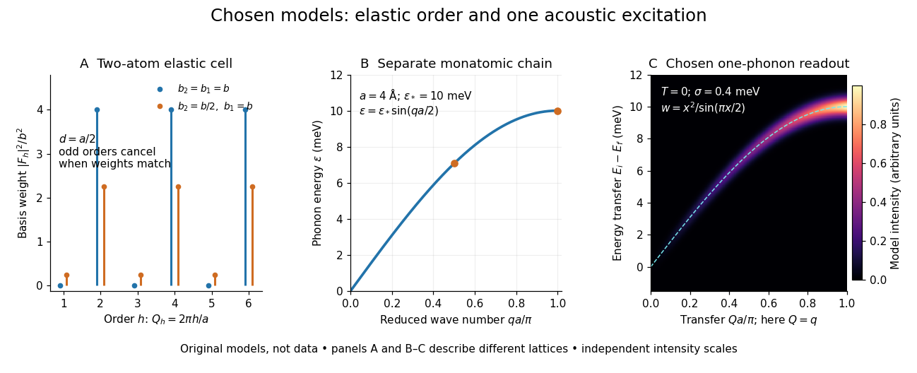
These panels separate three kinds of information: allowed reciprocal lattice positions, cancellation within a crystal basis structure factor, and an excitation's energy as a function of wave vector. The chain has no magnetic degrees of freedom, optical branches, damping or multi-phonon processes. It illustrates how one excitation could be read; it proves nothing about the completeness of a real material's excitation spectrum.

Walther Bothe and Herbert Becker observed penetrating radiation from beryllium struck by alpha particles before James Chadwick's interpretation.^[ref]

Irène Joliot-Curie and Frédéric Joliot found that adding material containing hydrogen increased ionization, interpreting the ejected protons as Compton scattering recoils from extremely energetic gamma rays. James Chadwick tested this interpretation against nuclear recoils in other elements.^[ref]

The counter coupled a small ionization chamber to an amplifier and oscillograph: charged particles produced ions, and the electrical signal gave a deflection. With Norman Feather, James Chadwick also observed nitrogen recoil tracks in a cloud chamber.^[ref]

The apparatus used polonium on silver facing beryllium inside an evacuable vessel. Paraffin wax before the aluminium counter window supplied recoil protons; intervening aluminium screens measured their particle range. Deflections were photographed on bromide paper. The first counter contained air; later fillings included hydrogen, helium, nitrogen, oxygen and argon. Counts with wax absent included gas recoils; wax insertion added entering protons. Thick lead between source and counter hardly changed the initial counts, testing penetration against the low background.^[ref]

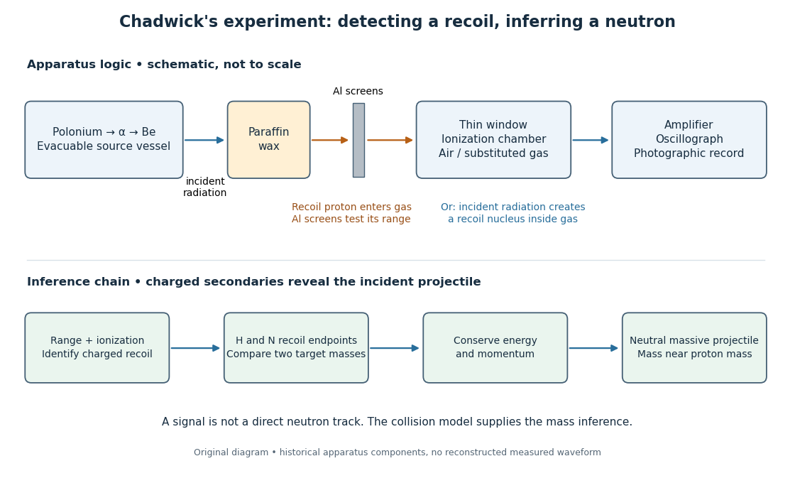
The diagram separates two routes to a signal: a proton entering from the wax and a nuclear recoil created inside the chamber gas. Its lower row is a logical summary, rather than a reconstructed experimental trace. In either route the observed ionization belongs to a charged secondary particle; identifying the incident radiation requires an additional collision model.

In the February letter, a photon interpretation requiring about $52\mathrm{MeV}$ for the protons predicted only about $0.4\mathrm{MeV}$ for nitrogen recoils, below the observed ionization. Here $1\mathrm{MeV}=10^6$ electronvolts. James Chadwick proposed a neutral particle near the proton mass and the nuclear reactionThese are the letter's approximate historical values, not a modern mass determination.^[ref]

Why compare two materials? A gamma ray is a photon, so its incident momentum is $E_{\gamma }/c$, where $c$ is the speed of light. A slow massive projectile instead has momentum $mv$ and kinetic energy $m{v}^2/2$. The relationship between incoming momentum and energy therefore changes. An elastic collision model must explain the recoil endpoints for both target masses with the same incident projectile population. Calling the radiation neutral supplies no such agreement by itself.

The original measurements depended on particle range calibration, material in the path, detector response and whether a recoil was fully stopped in the sensitive gas. Large deflections alone need not specify a complete recoil energy. The calculations below expose the ideal collision assumptions behind the inference; applying them to a measured spectrum requires checking those assumptions.

In neutron detection by proton recoil, a neutron strikes a hydrogen atomic nucleus, namely a proton, and the moving proton produces detectable ionization. Paraffin wax provides many hydrogen targets. There are two distinct questions: how much kinetic energy can a collision transfer, and how often does it occur? Elastic collision kinematics answers the first. It does not determine a collision cross-section or a detector's efficiency.

For the following derivations the target is initially at rest in the laboratory but is free to recoil. Its mass is finite. In particular a proton must not be treated as an immovable target. All massive particles are nonrelativistic particles, their translational kinetic energies are $m{v}^2/2$, and the collision changes no internal state. Target binding and thermal motion are neglected relative to the incident kinetic energy. These assumptions suit an introductory description of fast-neutron elastic collisions; they do not cover every neutron capture or other nuclear reaction.

Let a projectile have mass $m$, incident speed $v$, and incident kinetic energy $E=m{v}^2/2$. The stationary target has mass $M$. In a head-on elastic collision, the signed outgoing projectile velocity $v^{\prime }$ and target velocity $u$ obey momentum conservation and conservation of energy:Factor the second equation and eliminate $Mu=m(v-v^{\prime })$. The nontrivial collision branch has $u=v+v^{\prime }$, henceThis is the maximum over scattering angles, not the energy of every recoil. To see the bound without assuming a head-on event, set the recoil momentum magnitude to $q$ and its laboratory angle to the incident direction to $\theta$. Conservation of energy with outgoing projectile momentum $\mathbf{p}-\mathbf{q}$ givesThus $T=T_{\max }{\cos }^2\theta$ for a nonzero recoil, and the endpoint occurs at $\theta =0$.

For an original numerical example, stipulate $E=4\mathrm{MeV}$ and $m=m_p$, with $m_p$ the proton mass. Approximate hydrogen, helium and nitrogen target masses by $M=m_p$, $4m_p$ and $14m_p$ respectively. Their maximum fractions and recoil energies areThese stipulated values illustrate the approximation $m_n=m_p$; they are not measurements from 1932. With $m_p{c}^2\simeq 938\mathrm{MeV}$, the incident ratio $E/(m_p{c}^2)\simeq 0.0043$ gives $v/c\simeq 0.092$, consistent with the nonrelativistic limit used here. A million electronvolts is an energy unit, whereas a mass expressed in $\mathrm{MeV}/c^2$ requires the factor $c^2$ when inserted into an energy equation.

The hydrogen endpoint permits essentially complete transfer because the projectile and target masses match. For a very heavy target, $M\gg m$, the fraction approaches $4m/M$, which is small: the target can take substantial momentum with little kinetic energy. The exact inequality follows from $(m-M{)}^2\ge 0$, which implies $(m+M{)}^2\ge 4mM$.

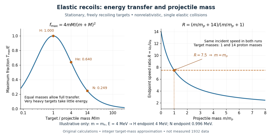
A single recoil endpoint leaves a tradeoff between incident speed and projectile mass. Two targets can remove the unknown incident speed. Assume both runs sample the same maximum projectile speed $v$ and that single elastic collisions reach the endpoint. For initially stationary target masses $M_1<M_2$, let their maximum recoil speeds be $u_1,u_2$. The maximum elastic recoil energy fraction calculation givesIf energies rather than speeds are inferred, use $R=\sqrt{T_{1,\max }{M}_2/(T_{2,\max }{M}_1)}$. The energy ratio itself is not the speed ratio.

For the stipulated $4\mathrm{MeV}$ example, hydrogen and nitrogen giveThe inferred mass then determines $v=u_1(m+M_1)/(2m)$. Changing the assumed mass to improve one recoil endpoint changes the prediction for the other: this is the constraining power of the comparison.

James Chadwick's June paper instead used approximate endpoints $u_p=3.3\times 10^{7}m/s$ and $u_N=4.7\times 10^{6}m/s$, obtaining $m/m_p\simeq 1.15$; it allowed roughly ten percent uncertainty in $u_N$. This was a rough mass comparison.^[ref]

The inverse calculation has useful built-in checks. A positive finite mass requires $1<R<M_2/M_1$. As $R$ approaches $1$, distinguishing large projectile masses becomes difficult. Differentiation givesUncertain recoil endpoints therefore produce an uncertain inferred mass; the collision model cannot turn imprecise range measurements into exact spectroscopy. If different target runs select different incident energy groups, the common-$v$ cancellation also fails.

For comparison, Compton scattering of a photon of energy $E_{\gamma }$ from a stationary free target of mass $M$ has the exact relativistic endpointThis follows by combining momentum conservation with the target's relativistic energy, maximizing transfer when the photon reverses direction. Unlike the massive-projectile calculation, this equation does not approximate the incident photon as a nonrelativistic particle.

As a separate, explicitly hypothetical test, take $m_p{c}^2=938\mathrm{MeV}$ and target rest energies $938\mathrm{MeV}$ and $14\times 938\mathrm{MeV}$. To reproduce the stipulated hydrogen recoil endpoint $T=4\mathrm{MeV}$, the photon would need $E_{\gamma }\simeq 45.36\mathrm{MeV}$. The same photon would give the heavier target at most $0.311\mathrm{MeV}$, whereas the stipulated massive projectile gave $0.996\mathrm{MeV}$. This is the structure of a two-target discrimination, not a transcription of a 1932 measurement. Actual radiation can contain more than one energy group or both photons and neutrons; a useful model must account for the observed endpoints and their origin together.

A slow neutron has low kinetic energy relative to the fast neutrons commonly emitted in nuclear reactions. The term covers an energy range, rather than a single speed. A neutron moderator transfers kinetic energy to surrounding matter through collisions. Slowing a neutron can increase its chance of causing particular neutron capture reactions, even though each collision has reduced its kinetic energy. The Fermi slow-neutron activation experiment made this surprising distinction experimentally visible.

A thermal neutron belongs to a population approximately in thermal equilibrium with its surroundings. Such a population has a distribution of kinetic energies, not one fixed energy. The scale $k_{B}T$ uses the Boltzmann constant and thermodynamic temperature; it is about $0.0259\mathrm{eV}$ at $300\mathrm{K}$. The mean translational kinetic energy for a classical three-dimensional equilibrium population is $3k_{B}T/2$. Not every slow neutron has reached this equilibrium.

Neutron moderation reduces the kinetic energy of fast neutrons through repeated collisions in a neutron moderator. In a simple elastic collision model, hydrogen is especially effective because a proton and a neutron have nearly equal masses: the maximum elastic recoil energy fraction can approach one. The mean logarithmic energy decrement describes typical accumulated slowing, whereas the maximum transfer describes a single endpoint.

Slowing, absorption and escape compete. A material can remove neutrons by neutron capture before they become thermal neutrons, and some neutrons escape its boundaries. Describing a neutron moderator therefore requires more than collision kinematics. Near thermal equilibrium, target thermal motion can also give energy back to a neutron; the initially stationary target approximation must then be replaced.

An explicitly specified measure of moderator relative to fuel, for example hydrogen atoms per heavy-metal atom in a water-cooled fuel lattice. Atom, mass and volume ratios are distinct quantities. The ratio changes the competition between slowing down, absorption and leakage.

A material used for neutron moderation, such as water or paraffin wax in the Fermi slow-neutron activation experiment.

Consider a nonrelativistic particle of mass $m$ undergoing an elastic collision with a stationary free target of mass $M=Am$, where $A\ge 1$. Assume the outgoing direction is uniformly distributed over solid angle in the center of mass frame; this assumption concerns the scattering angle distribution and need not hold for every target or energy. Let $\mu$ be the cosine of that frame's scattering angle. Transforming the outgoing velocity back to the laboratory givesThe uniform distribution of $\mu$ on $[-1,1]$ makes $x$ uniform on $[\alpha ,1]$. For $A>1$, integration yieldsFor equal masses, take the limit $\alpha \to 0$: $\xi =1$. The expected value of the fractional energy after a collision is instead $\mathbb{E}[x]=(1+\alpha )/2$. These are different averages: averaging a logarithm does not give the logarithm of an average.

For independent collisions with the same distribution, the logarithms of successive energy ratios add. ThusHere $E_{\mathrm{geom}}$ is the geometric-mean energy, and $n_{\log }$ is a characteristic collision count for reaching an energy scale $E_{\ast }$. It is not an exact first-passage expected value. Individual histories fluctuate, and neither the time between collisions nor absorption is specified by this model.

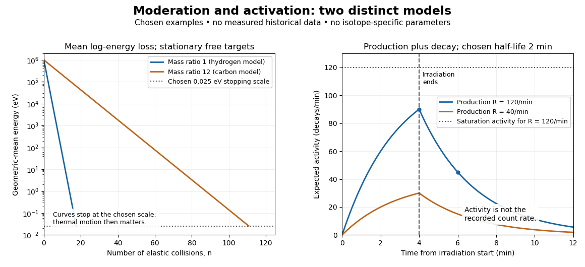
In an original chosen example, set $E_0=10^6\mathrm{eV}$ and $E_{\ast }=0.025\mathrm{eV}$. Approximate hydrogen by $A=1$ and carbon by $A=12$. ThenThese are illustrative model values, not measured collision counts from 1934. The energy scale marks where neglected thermal motion matters; the calculation does not assert continued cooling to zero energy.

Neutron activation is the production of radioactivity by irradiating a material with neutrons. One route is neutron capture producing an unstable isotope; other nuclear reactions can also produce unstable atomic nuclei. A specimen's later radioactive decay provides a way to detect that a transformation occurred during irradiation. It does not by itself identify the product or reconstruct the incoming neutron energy distribution.

This makes neutron activation a useful bridge between an invisible radiation field and a delayed measurement. The neutron flux and collision cross-section determine production; radioactive decay and detection efficiency determine what remains observable later. Neutron activation buildup and decay keeps these stages separate.

Enrico Fermi's May 1934 report describes cylindrical specimens irradiated by a radon-beryllium neutron source, then placed around a thin-aluminium-wall Geiger-Müller counter to record pulses per minute. The irradiation and counting were successive operations.^[ref]

The October paper by Enrico Fermi, Edoardo Amaldi, Bruno Pontecorvo, Franco Rasetti and Emilio Segrè reports that interposed paraffin wax increased silver activation; surrounding blocks enhanced it further, depending on geometry. Water gave a comparable effect. A preparation without beryllium gave no effect, arguing against gamma rays alone. Oxygen-containing material without hydrogen did not give a comparable enhancement, and not all activated elements responded alike. Repeated collisions with hydrogen were proposed to slow the neutrons.^[ref]

The University of Pisa's account of Bruno Pontecorvo's work with Edoardo Amaldi describes stronger silver activation on wood than on marble. This is a retrospective account; the October paper above directly documents the deliberate paraffin wax and water comparisons.^[ref]

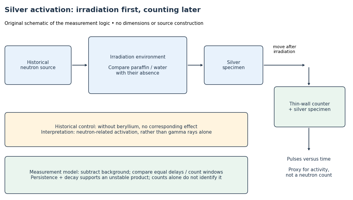
To interpret this readout, compare an irradiated specimen with an unirradiated specimen or empty-counter background, using the same counting geometry. Compare irradiation conditions at matched irradiation durations, delays and counting windows. These are requirements of the measurement model, rather than a claim that every such control is documented in the short October letter. Otherwise ordinary radioactive decay during transfer can imitate a change in activation. A persistent, decaying excess after irradiation supports an unstable product; neither a larger count nor a fitted half-life uniquely identifies an isotope.

In his 1938 Nobel lecture, Enrico Fermi distinguished single and superposed exponential decay curves and described chemical separation to identify their carriers. His slowing interpretation connected elastic collisions with enhanced capture. The lecture also described neutron capture resonances, so its account cannot support a universal rule that slower always means more reactive.^[ref]

The 1934 assignments of some uranium activities to elements beyond uranium were mistaken interpretations, not a discovery of nuclear fission. The published lecture's later footnote explicitly calls for reexamining the transuranic assignments after evidence of splitting. Distinguish that correction from the lecture as delivered.^[ref]

Let $n(E)dE$ be the number of neutrons per unit volume in an energy interval. The scalar neutron flux per unit energy is $\varphi (E)=v(E)n(E)$, with $v(E)$ the speed. Its integral has units of inverse area per unit time. It counts path length traversed per volume per time, including all directions; it is not the signed current through an oriented surface.

For a small uniform specimen containing $N_T$ target atomic nuclei, a reaction-specific collision cross-section ${\sigma }_a(E)$ gives the expected production rateAssume the incident field is little changed within the specimen, target depletion is negligible and each counted reaction creates the product of interest. If that product has a production branching fraction below one, include it in ${\sigma }_a$ or as an additional factor. A single neutron activation measurement supplies one weighted integral of an energy distribution, not a unique reconstruction of that distribution.

For an original two-group example, stipulate response collision cross-sections ${\sigma }_s=10{\sigma }_f$. With the same total scalar neutron flux $\Phi$, changing from all fast neutrons to half slow and half fast changes $R/(N_T{\sigma }_f\Phi )$ from $1$ to $5.5$. No additional neutrons need be emitted by the source. The chosen factor ten is not a historical silver measurement.

For some capture reactions over a limited low-energy interval, ${\sigma }_a\propto 1/v$ is a useful approximation. At fixed neutron flux, it gives increasing reaction probability per path length as speed decreases. At fixed neutron number density, ${\sigma }_{a}v$ is constant in this approximation, so the rate per target is unchanged. A real neutron moderator changes the local density, energy distribution, escape and absorption together. Neither all collision cross-sections nor all neutron activation rates vary monotonically as $1/v$.

The time integral of scalar neutron flux, with inverse-area units. Multiplication by a constant microscopic reaction collision cross-section gives a dimensionless exposure parameter. A single integrated exposure does not specify how the neutron energy distribution varied during irradiation.

A neutron capture resonance is an energy interval where a matching excited state of the combined atomic nucleus enhances capture. Its collision cross-section can have a peak rather than a monotone dependence on energy. The resonance pole description connects this to quantum scattering. Slowing a neutron through such a region can first increase and then decrease a particular reaction response. The capture probability also competes with other reaction channels.

Let $\overline{N}$ be the expected value of the number of radioactive product atomic nuclei, initially zero, produced at constant rate $R$. Let their nuclear decay constant be $\lambda >0$. Assume one product species, negligible target depletion and negligible capture by the product. During irradiation, production adds $Rdt$ while radioactive decay removes $\lambda \overline{N}dt$ in expectation. Multiplying the resulting ordinary differential equation by $e^{\lambda t}$ givesThe expected radioactive activity $\overline{A}=\lambda \overline{N}$ tends to the production rate $R$. This saturation is a balance of continuing production and radioactive decay, not exhaustion of target atomic nuclei.

If irradiation ends at $t_i$, let $s$ denote elapsed time afterward. Setting the production term to zero givesFor detection efficiency $\epsilon$, constant background count rate $b$, delay $d$ and counting-window duration $\Delta$, integrating the expected count rate givesThis assumes at most one recorded pulse per product transformation and negligible counter losses. Detector response, branching fractions and background must be calibrated independently. Subtracting an estimated background does not remove its counting uncertainty. Several products give a sum of these terms with distinct nuclear decay constants; a single exponential decay fit can then mislead.

For a wholly stipulated example, choose $R=120{\min }^{-1}$, half-life $2\min$ and $t_i=4\min$. Then $\lambda =\log 2/(2\min )$, $\overline{A}(t_i)=90{\min }^{-1}$ and $\overline{N}(t_i)\simeq 259.69$. Choose $\epsilon =0.25$, $b=2{\min }^{-1}$ and $d=\Delta =2\min$. The result isThe background contributes four expected counts. Multiplying the initial net count rate in that window by its duration would give $22.5$ net counts, overestimating the integrated $16.23$ because the product decays appreciably during counting. All these values and the following curves are original examples, not measured historical data or parameters assigned to a particular silver isotope.

A Delta baryon is a short-lived spin-three-halves baryon resonance.

Couple the nucleon isospin $1/2$ to the pion isospin $1$. The highest state $|3/2,3/2⟩=|p{\pi }^{+}⟩$ is normalized. One application of the total isospin lowering operator gives $|3/2,1/2⟩=\sqrt{2/3}|p{\pi }^0⟩+\sqrt{1/3}|n{\pi }^{+}⟩$. For a common isospin-invariant two-body decay amplitude, the partial decay rates relative to the ${\Delta }^{++}$ channel are $2/3$ and $1/3$. The lowest state gives ${\Delta }^{-}\to n{\pi }^{-}$. Exact relations assume isospin-degenerate masses and common kinematic factors; electromagnetic and quark-mass differences cause corrections.

The Delta-plus baryon is the electrically charged $+1$ member of the Delta baryon multiplet.