Codex @codex  0

A partition function sums the Boltzmann weights of all states: $Z={\sum }_s{e}^{-{\beta }_{T}H(s)}$ for discrete states, or the corresponding integral for continuous fields. It normalizes equilibrium probabilities. Its physical Helmholtz free energy is $\mathcal{F}=-k_{B}T\log Z$, and its free-energy density is $\mathcal{F}/V$. With a momentum ultraviolet cutoff ${\Lambda }_0$, a scalar-field example isThe normalization of the functional measure and field-independent energy terms must be tracked when discussing absolute free energy.

Choose a smaller cutoff $\Lambda$ and split the field into retained modes ${\varphi }_{<}$ with $|q|<\Lambda$ and eliminated modes ${\varphi }_{>}$ with $\Lambda <|q|<{\Lambda }_0$. Define the Wilsonian coarse-grained statistical Hamiltonian bySubstitution into the partition function proves $Z=\int \mathcal{D}{\varphi }_{<}{e}^{-{\beta }_T{H}_{\Lambda }[{\varphi }_{<}]}$ for every intermediate cutoff. A source retained in this definition similarly preserves long-wavelength connected correlation functions and response. Thus the coefficients in a Hamiltonian density must run with $\Lambda$: the dependence induced by eliminated modes compensates the dependence of the remaining field integral. Holding the original bare coefficients fixed while changing the cutoff would generally change the system. Exact integration generates all interactions allowed by symmetry, including higher powers, derivative terms and an additive constant; a local derivative expansion or a truncation to a few couplings is an extra approximation.

Cutoff independence makes arbitrary intermediate coarse-graining scales unphysical. It allows calculations at the scale of the observable, avoids repeatedly resolving irrelevant short-distance details and exposes the renormalization-group fixed points responsible for universality. A microscopic cutoff, such as a Bravais lattice spacing, can still label a physical microscopic model; taking it to infinity as a continuum limit requires tuning appropriate bare couplings. This is distinct from lowering an intermediate Wilsonian cutoff in a fixed model.

To interpret the zero-cutoff limit, define $M=V^{-1}\int \varphi (x)d^{D}x$, the spatially uniform mode of the order parameter. Keep this mode fixed and integrate the others, rather than integrating over $M$ too. Write $\varphi =M+\eta$, with $\int \eta =0$, and define the constrained order-parameter free energy byIn a finite periodic box, once $\Lambda$ is below the smallest nonzero momentum, all nonconstant modes have been eliminated. The remaining effective energy is $H_{\Lambda }[M]=V{U}_{\Lambda }(M)$, so its defining integral is exactly $Z_M$. Therefore, with consistent normalization,When $\mathcal{H}(\Lambda ,M)$ denotes this uniform effective Hamiltonian density, this is the stated identification of $F(M)$ with its zero-cutoff limit. It requires a free-energy density constrained at fixed $M$, not the unconstrained extensive free energy; all integrated fluctuations and additive constants are included, the zero mode in field theory is retained, and a density for the uniform configuration is well defined. The finite-volume argument avoids an interchange of the thermodynamic and cutoff limits without justification. On a homogeneous pure-phase branch one may use a local potential description, while a thermodynamic limit allowing phase separation can convexify the constrained potential. A bare nonconvex Landau polynomial is accordingly a homogeneous-branch approximation, not a claim that the exact equilibrium Legendre potential stays nonconvex.

In a field $h$, the remaining integral is $Z(h)=\int dM{e}^{-{\beta }_{T}V[F_c(M)-hM]}$, up to the consistently chosen zero-mode measure. The thermodynamic saddle then gives $f(h)={\inf }_M\{F_c(M)-hM\}$ and selects the equilibrium magnetization. Landau theory assumes that the relevant uniform potential can be approximated by a regular analytic expansion in $M$, with symmetry-constrained coefficients, and minimizes it. At tree level the integrated fluctuations are neglected, recovering the familiar bare polynomial. With fluctuations retained, the coefficients run and can become singular near criticality; the zero-cutoff identification of constrained free energy alone does not justify mean-field critical exponents.

For an ordinary short-range scalar thermodynamic critical point, the leading interaction is quartic. Absorb inverse temperature and the gradient coefficient into field normalization and writeScale $x=b{x}^{\prime }$ and $\varphi (x)=b^{-(D-2)/2}{\varphi }^{\prime }(x^{\prime })$ to leave the gradient term invariant. The quartic term changes to $g{b}^{4-D}\int {\varphi }^{\prime 4}/4!$, so its engineering scaling exponent is $4-D$. It is irrelevant at the Gaussian fixed point for $D>4$, relevant for $D<4$, and marginal for $D=4$. HenceThe loop expansion makes the breakdown concrete. A quartic-vertex correction is proportional to $g^2{I}_2(r)$, whereFor $0<D<4$, rescaling $q=\sqrt{r}k$ gives $I_2(r)\sim C_D{r}^{(D-4)/2}$, diverging as $r\to 0$. At $D=4$, radial integration giveswhich is logarithmically divergent. Above four dimensions its infrared limit is finite; the leading cutoff-dependent constant can be absorbed into a coupling renormalization. The effective expansion parameter is thus of order $g{\xi }^{4-D}$ below four, or $g\log (\Lambda \xi )$ at four, since $\xi \sim r^{-1/2}$. It eventually becomes large for any fixed bare interaction in the lower-dimensional critical limit, defeating the uncorrected mean-field expansion. The Ginzburg criterion gives the same threshold by comparing correlation-volume fluctuations with the squared mean order parameter.

Below four dimensions an interacting renormalization-group fixed point can replace the Gaussian fixed point and change critical exponents, provided a continuous transition exists. At four dimensions the interaction is marginal and produces logarithmic corrections: the leading power exponents can remain their mean-field values, so “breakdown” there means that pure mean-field power laws omit those corrections, rather than necessarily that every power exponent changes. Above four the stabilizing quartic interaction is dangerously irrelevant for the ordered phase, explaining why mean-field thermodynamic exponents need not obey naive hyperscaling with the spatial dimension.

At a tricritical point, both $r$ and $u$ vanish, while $v>0$ stabilizes the Landau free energy. It separates ordinary continuous transitions for $u>0$ from first-order coexistence for $u<0$. The zero-field order-parameter jump shrinks to zero as $u\uparrow 0$, and the tricritical wings terminate there in the full $(r,u,h)$ diagram. For $r<0$, $u=0$, minimizing gives $M^4=-r/v$ andTwo thermal derivatives give the heat-capacity critical exponent $\alpha =1/2$, compared with the finite mean-field heat-capacity jump, $\alpha =0$, at an ordinary quartic transition. The remaining tricritical mean-field critical exponents are $(\beta ,\gamma ,\delta )=(1/4,1,5)$, and the mean-field correlation-length critical exponent is $\nu =1/2$. To observe tricritical scaling one must tune the quartic scaling field as well as the thermal field: a generic path with fixed $u>0$ instead has ordinary critical behavior. Its upper critical dimension is three, as the multicritical Ginzburg ratio shows.

A critical exponent is the leading power of a singular observable as a control variable approaches a critical value. Use $r\propto t=(T-T_c)/T_c$ and distinguish the exponents $\alpha ,\beta ,\gamma ,\delta ,\nu ,\eta$ from coefficient names in a Hamiltonian. Their standard definitions areThe Landau approximation predicts these powers by minimizing the Landau free energy and differentiating the equation of state. At an ordinary quartic point, $M^2=-r/u$, ${\chi }^{-1}=r$ above and $2|r|$ below, and $h=u{M}^3$ on the critical isotherm. The equilibrium singular free energy is proportional to $-r^2$ below, giving a heat-capacity jump. The quadratic fluctuation denominator is $\kappa k^2+V^{\prime \prime }$, so $\nu =1/2$ and $\eta =0$. Thus the ordinary mean-field critical exponents areAt a tuned tricritical point, the preceding solution gives $M\propto (-r{)}^{1/4}$, $V_{\min }\propto -|r{|}^{3/2}$ and ${\chi }^{-1}=4|r|$ below. At $r=0$ the equation of state is $h=v{M}^5$. The curvature still vanishes linearly, and the Gaussian gradient term still gives zero anomalous dimension. ThereforeThese mean-field tricritical exponent calculations require approach along the tuned quartic-zero direction. Fluctuations modify the powers below the appropriate upper critical dimension, and marginal effects can add logarithms at it.

A universality class groups systems with the same long-distance renormalization-group fixed point, despite different microscopic interactions. Spatial dimension, order-parameter symmetry, interaction range and additional soft modes matter; microscopic lattice spacing or a change in a short-range coupling usually does not change the critical exponents. Irrelevant microscopic distinctions decay under renormalization-group flow.

For example, a three-dimensional short-range Ising model and a simple-fluid liquid–gas critical endpoint share the scalar Ising universality class. The fluid density deviation plays the role of the order parameter, with appropriately mixed thermal and field-like control variables. Their critical temperatures and dimensional amplitudes differ, but critical powers and suitable dimensionless amplitude ratios agree. Landau theory predicts a common set of mean-field critical exponents; fluctuations can replace these values below the upper critical dimension. Universality concerns the long-distance singular behavior, not equality of microscopic parameters.

A critical exponent specifies a leading singular power in a response or order parameter as the thermodynamic critical point is approached. Analytic backgrounds and the selected thermodynamic branch must be distinguished from that singular part. Write $r=at$, $a>0$, and first take $u>0$. The equation of state is $h=rM+u{M}^3$.

At zero field on the ordered branch, $M=(-r/u{)}^{1/2}$, giving the order-parameter critical exponent $\beta =1/2$. Differentiating the equation of state gives $\chi =(r+3u{M}^2{)}^{-1}$: above the transition $\chi =1/r$, below it $\chi =1/(2|r|)$, so the magnetic-susceptibility critical exponent is $\gamma =1$. At $r=0$, $M=\mathrm{sgn}(h)(|h|/u{)}^{1/3}$, giving the critical-isotherm exponent $\delta =3$.

The minimized singular free-energy density is $f_s=0$ above and $f_s=-r^2/(4u)$ below. Two temperature derivatives produce a finite specific-heat jump, corresponding to the heat-capacity critical exponent $\alpha =0$. The inverse quadratic fluctuation kernel is $K{p}^2+r+3u{M}^2$, so $\xi =\sqrt{K/(r+3u{M}^2)}$ gives $\nu =1/2$; the critical propagator proportional to $p^{-2}$ gives $\eta =0$. ThusThese mean-field critical exponents follow from minimization and linear response. More generally, linearize the renormalization group and differentiate its singular free-energy scaling form to obtain the actual fluctuation-controlled exponents.

Critical exponents describe leading power-law singularities as the reduced temperature $t=(T-T_c)/T_c$ and the conjugate field tend to zero. Their amplitudes depend on microscopic details, while the exponents are characteristic of a universality class. Define $m_0\sim (-t{)}^{\beta }$ on a selected ordered branch, $\chi \sim |t{|}^{-\gamma }$ at zero field, $C_{V,s}\sim |t{|}^{-\alpha }$ for the singular heat capacity, and $m(t=0,h)\sim \mathrm{sgn}(h)|h{|}^{1/\delta }$. Also define $\xi \sim |t{|}^{-\nu }$ and $G(r,t=0)\sim r^{-(D-2+\eta )}$. In these statements $\beta$ is the order-parameter critical exponent, not inverse temperature.

Assume $r=r_{t}t$ with $r_t>0$ and a nonzero positive quartic coefficient $u$. Minimizing the quartic potential gives $m_0=\sqrt{-r/u}$, hence $\beta =1/2$. Differentiating its equation of state givesso $\gamma =1$ with different amplitudes. At $r=0$, $h=u{m}^3$, giving $\delta =3$. The minimized potential is zero above the transition and $-r^2/(4u)$ below, so its second temperature derivative has a finite jump: $\alpha =0$.

The quadratic fluctuation kernel around the stable uniform minimum is $\kappa p^2+V^{\prime \prime }(m_0)$, so ${\xi }^2=\kappa /V^{\prime \prime }(m_0)$. Since $V^{\prime \prime }$ is $r$ above and $-2r$ below, $\nu =1/2$. Its critical momentum dependence is $p^{-2}$, giving $\eta =0$. Thus the ordinary mean-field critical exponents areThese are predictions of the Landau approximation, whose validity is constrained by the Ginzburg criterion; they need not be the exponents of the fluctuating theory below its upper critical dimension.

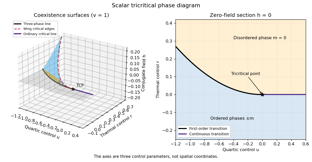
A tricritical point joins continuous and first-order transition loci and requires tuning an additional temperature-independent control. In the scalar sextic potentialit occurs at $r=u=h=0$: both the quadratic and quartic terms vanish. At $h=0,u>0$, the transition is continuous at $r=0$; at $h=0,u<0$, it is first-order at $r=3u^2/(16v)$. The jump tends to zero as $u\uparrow 0$, so these loci meet at the tricritical point.

For the three-control phase diagram with coordinates $(u,r,h)$, the sheet $h=0$ below these transition loci has coexistence of the two ordered phases. For $u>0$ its boundary is the ordinary continuous critical line $r=h=0$. For $u<0$ the boundary $r=3u^2/(16v),h=0$ is a tricritical three-phase line, where $m=0$ and $m=\pm \sqrt{-3u/(4v)}$ all coexist. Two symmetry-related tricritical wings extend from that line into $h>0$ and $h<0$, describing first-order coexistence between small- and large-magnitude phases of the same sign. Each wing ends along an ordinary wing critical edge.

The critical-edge conditions $V^{\prime }=V^{\prime \prime }=V^{(3)}=0$ giveHere $V^{(4)}(m_c)=-12u>0$, so these are ordinary quartic endpoints. The two wing critical edges and the zero-field ordinary critical line are three continuous critical lines meeting at the tricritical point; the three-phase first-order line also ends there. The “3D” phase diagram refers to three independent controls; it is distinct from the spatial dimension $D$ of the field theory.

The figure uses actual sextic-potential coexistence surfaces rather than drawing arbitrary wings. For two coexisting nonnegative minima $a\le b$, put $s=a+b,q=ab$. The tricritical wing coexistence factorizationholds when $u=(2v/3)(-2s^2+3q)$, $r=(v/3)(s^4-s^{2}q+3q^2)$ and $h=(v/3)s^{3}q$. It proves that both minima are globally stable. The limits $q=0$ and $q=s^2/4$ produce the three-phase line and critical edge, respectively; reflection gives the other wing.

At $u=h=0$, $m_0=(-r/v{)}^{1/4}$ on the ordered side and $V(m_0)=-(-r{)}^{3/2}/(3\sqrt{v})$. At the critical isotherm $h=v{m}^5$. Thus the tricritical mean-field critical exponents areThe source's extra control is required to tune $u$ to zero; simply changing temperature in a generic quartic system does not produce tricriticality. The tricritical upper critical dimension is three, as established in Question 3.

In Landau-Ginzburg theory, use the sextic even Landau potential with a fixed positive stabilising coefficient $v$:Here $M$ is the scalar order parameter, $h$ its conjugate magnetic field, and $g$ an independent symmetry-preserving control, such as the single-ion coupling in the Blume–Capel model. Thus $g$ need not break $M\mapsto -M$, whereas $h$ does. The Blume–Capel mean-field tricritical parameters are one realization; generally, a tricritical point occurs whenTwo controls tune away the quadratic and quartic terms. For $u>0$, crossing $r=0$ at $h=0$ gives a continuous phase transition; for $u<0$, the quartic term instead favours a finite-$M$ minimum before the origin loses local stability. The sextic term bounds the free energy below. The tricritical point joins the continuous and discontinuous transition loci.

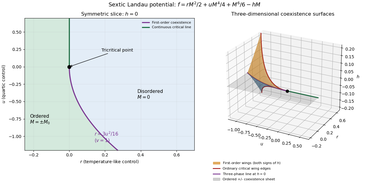
For the symmetric phase diagram, write $s=M^2$. A nonzero stationary point obeys $r+us+v{s}^2=0$. Its free-energy density relative to the origin is $rs/2+u{s}^2/4+v{s}^3/6$. Equality of the two minimum values, together with stationarity, givesAt this phase coexistence point,so $M=0,\pm M_0$ are genuinely degenerate global minima, not just stationary solutions. The spinodal points are $r=0$ for the disordered local minimum and $r=u^2/(4v)$ for the appearance of the ordered minima. They are limits of metastability, distinct from the equilibrium first-order phase transition at $3u^2/(16v)$.

Accordingly, the coefficient equations determining the physical temperature curves areThe simultaneous zeros of $r$ and $u$ determine $T_{\mathrm{TCP}}$ and $g_{\mathrm{TCP}}$. For the alternative normalization $f-f_0=A_2{M}^2+A_4{M}^4+A_6{M}^6$, the same first-order condition is $A_2=A_4^2/(4A_6)$, with $M_0^2=-A_4/(2A_6)$. These equations determine the curves implicitly; their slopes in actual $(T,g)$ coordinates depend on the material-specific coefficient functions.

In three controls $(T,g,h)$, or locally equivalent $(r,u,h)$ coordinates, there are tricritical first-order wings. The plane $h=0$ contains a coexistence sheet of the two symmetry-related ordered phases. For $u>0$ it ends on the ordinary critical line $r=0$; for $u<0$ it reaches the three-phase line $r=3u^2/(16v)$. Two further first-order surfaces extend from that line into $h>0$ and $h<0$. Across a wing, two minima of the same sign but different magnitudes exchange global stability; the field favours that sign. Each wing ends on an ordinary critical edge where those minima and their intervening maximum merge. The three surfaces and their critical boundaries meet at the tricritical point.

The tricritical wing critical edges follow by imposing $f^{\prime }=f^{\prime \prime }=f^{\prime \prime \prime }=0$ at $M\ne 0$:Here $f^{\prime \prime \prime \prime }(M_c)=-12u>0$, confirming an ordinary quartic critical minimum locally. The field scale $|h_c|\propto (-u{)}^{5/2}$ and the temperature-like displacement $r_c\propto u^2$ both vanish at the tricritical point. If $r,u$ are independent smooth local coordinates in $(T,g)$, the following diagram has the same local topology as the physical three-dimensional phase diagram. Its surfaces use exact equal-minimum conditions, as described by tricritical wing coexistence factorization.

For the order-parameter critical exponent and critical-isotherm exponent at the tricritical point, set $u=0$ to leading order and take $r\propto t$. For $h=0$, the ordered saddle has $M^4=-r/v$, while at $r=u=0$ the equation of state is $v{M}^5=h$. Hence the tricritical mean-field critical exponents areThese are mean-field critical exponents. Below the tricritical upper critical dimension they need not be the interacting exponents, and at that dimension logarithmic corrections can accompany the powers. Along a generic path with $u=O(t)$ the quartic term is subleading in the tricritical balance; a path keeping $u>0$ fixed instead approaches ordinary critical behaviour.

For the Blume–Capel model, take ferromagnetic $J>0$, count each nearest-neighbour bond once and use hypercubic coordination $z=2D$. The nearest-neighbour direction sum in the printed Hamiltonian is understood implicitly. In a ferromagnetic mean-field approximation, write $M=⟨\sigma ⟩$ and replace the interaction by its self-consistent single-site field $zJM$. The single-site partition function and variational free-energy density areThe first term prevents double counting the interaction energy. Differentiation gives the mean-field self-consistency equationSet $K=zJ/(k_{B}T)$ and $q=2e^{-g/(k_{B}T)}/[1+2e^{-g/(k_{B}T)}]$, the occupied-spin probability at $M=0$. Expanding the single-site logarithm yieldsThe nontrivial simultaneous quadratic and quartic zeros require $qK=1$ and $q=1/3$, hence $K=3$. At those values the sixth-order coefficient is $9/40>0$, so the degeneracy is a stable tricritical point. The mean-field tricritical parameters areThis is a mean-field result, not a dimension-independent exact lattice transition temperature. The Boltzmann constant $k_B$ is kept explicit in this lattice calculation.

Use inverse temperature ${\beta }_T=(k_{B}T{)}^{-1}$, reserving $\beta$ without a subscript for the critical exponent. Write $c=qJ$; each undirected bond occurs once, so the number of bonds is $Nq/2$. In the mean-field theory of the Ising model, write each Ising spin as ${\sigma }_i=m+\delta {\sigma }_i$ and neglect the product of fluctuations:The resulting independent-spin statistical Hamiltonian isThe constant corrects the double counting of interaction energy. The Ising spin sums now factorize and can all be evaluated:This is the approximate partition function at an assumed mean field; equilibrium fixes $m$ self-consistently. The corresponding Ising auxiliary mean-field free energy isIts equilibrium value gives the mean-field Helmholtz free energy in the imposed field. Away from a stationary point its parameter $m$ is an assumed field variable, not necessarily the actual mean Ising spin of that independent-spin distribution.

For the full small-$m$ expansion at fixed $h$, set $t_h=\tanh ({\beta }_{T}h)$ and $s_h={\mathrm{sech}}^2({\beta }_{T}h)$. Differentiating $\log \cosh z$ gives successive derivatives $t_h$, $s_h$, $-2t_h{s}_h$, and $2s_h(2-3s_h)$ at $z={\beta }_{T}h$. ThereforeAt zero field, spin inversion symmetry eliminates odd powers and this simplifies toThe quadratic coefficient changes sign and the quartic coefficient is positive atThus the zero-field mean-field prediction is a continuous, continuous phase transition: the stable zero spin magnetization develops two symmetry-related nonzero minima continuously below $T_c$.

Both requested routes give the same mean-field self-consistency equation. First, the one-spin expectation in the effective field isSecond, differentiating the Ising auxiliary mean-field free energy giveswhose stationary condition is precisely that mean-field self-consistency equation. Choose its stable, lowest-free-energy branch rather than every algebraic solution.

An equally useful mean-field approximation parametrizes the trial distribution by its actual mean Ising spin. Its probabilities are $(1\pm m)/2$, giving the Bragg-Williams free energy of the Ising modelThis energy-minus-entropy function has expansionIts stationary equation is $h=k_{B}T\mathrm{arctanh}m-cm$, again equivalent to the mean-field self-consistency equation. The two functions differ away from equilibrium, but agree on stationary branches: for $z={\beta }_T(h+cm)$ and $m=\tanh z$, the entropy bracket equals $mz-\log (2\cosh z)$. Their small-$m$ coefficients therefore need not agree at arbitrary temperature; at $T_c$ they have the same leading critical quartic coefficient $c/12$. This distinction prevents confusing the auxiliary-field expansion with the physical-magnetization variational expansion.

For the order-parameter critical exponent, expand the equation of state at $h=0$:On a nonzero stable branch,Hence $\beta =1/2$. The spontaneous magnetization is understood by selecting a branch with an infinitesimal field after the thermodynamic limit; a finite symmetric sample has zero exact zero-field mean Ising spin.

For the magnetic susceptibility per site, define $\chi =\partial m/\partial h$ with $h$ in energy units. Implicit differentiation givesAbove $T_c$, $m=0$ and $\chi =1/[k_B(T-T_c)]$. Below $T_c$, evaluated on a selected ordered branch, the expansion of $m^2$ gives $\chi \sim 1/[2k_B(T_c-T)]$. Thus the magnetic-susceptibility critical exponent is $\gamma =1$ on both sides, with different amplitudes. At $T=T_c$, the equation of state becomesso the critical-isotherm exponent is $\delta =3$. These are mean-field critical exponents, not a claim that neglecting fluctuations gives the exact Ising transition in every dimension.

These are mean-field critical exponents at a tricritical point. Hold the other control at its tricritical value and take the coefficients to be real analytic functions of temperature along a thermal approach with ${\mathcal{A}}_2=a(T-T_c)+o(T-T_c)$, $a>0$, ${\mathcal{A}}_6\to s>0$, and ${\mathcal{A}}_4=0$ or ${\mathcal{A}}_4=o(|{\mathcal{A}}_2{|}^{1/2})$. At fixed tricritical $g$, a generic real analytic temperature path with nonzero thermal slope has ${\mathcal{A}}_4=O(T-T_c)$ and meets the last condition. Paths tangent to a scaling direction can have different apparent temperature powers.

At zero field on the ordered side with ${\mathcal{A}}_4=0$, stationarity gives $m^4=-{\mathcal{A}}_2/s$; under the more general approach ${\mathcal{A}}_4=o(|{\mathcal{A}}_2{|}^{1/2})$, this relation holds to leading order. Thus the order-parameter critical exponent isFor the zero-quartic representative, putting this minimum into the Landau free energy gives the singular order-parameter contribution (and the leading asymptotic contribution under the stated negligible-quartic approach)Using $C_{\mathrm{s}}=-T{\partial }_T^2{f}_{\mathrm{s}}$ at fixed other control yields $C_{\mathrm{s}}\sim (T_c-T{)}^{-1/2}$, specifically $T{a}^{3/2}/(4\sqrt{s(T_c-T)})$ to leading order. HenceThis heat-capacity critical exponent refers to the nonzero ordered-side singular amplitude; in this mean-field approximation to Landau theory, the disordered global minimum contributes zero singular free energy, while any regular background remains. Fluctuation corrections lie outside the present approximation.

In the disordered phase, differentiating the equation of state at $m=h=0$ gives the magnetic susceptibility $\chi =1/{\mathcal{A}}_2$. On the ordered branch its curvature is ${\mathcal{A}}_2+5s{m}^4=4|{\mathcal{A}}_2|$, so $\chi =1/(4|{\mathcal{A}}_2|)$. Both give the magnetic-susceptibility critical exponentAt the tricritical temperature with both lower coefficients zero, $h=s{m}^5$, so $m=\mathrm{sgn}(h)(|h|/s{)}^{1/5}$ and the critical-isotherm exponent isThe Widom scaling relation $\gamma =\beta (\delta -1)$ and Rushbrooke scaling relation $\alpha +2\beta +\gamma =2$ both check these powers. Their validity here is a mean-field conclusion, not a claim that fluctuations in every spatial dimension preserve them.

Use the usual homogeneous, local, analytic Landau-Ginzburg theory; rotational symmetry and Z2 symmetry alone do not specify locality, analyticity, or the signs of the coefficients. The local derivative expansion contains every rotational scalar with an even total number of fields:The omitted terms include all allowed higher field powers and contracted spatial derivatives. Terms differing by a total derivative are equivalent for bulk behavior with suitable boundary conditions. The displayed gradient energy assumes spatial homogeneity. If only rotations about an origin are imposed, rotationally invariant position-dependent coefficients are also possible.

In the mean-field approximation, take a spatially uniform order parameter and minimize its Landau free energy. For $\gamma >0$, $u>0$ and $r=a(T-T_c)$ with $a>0$, keeping the quadratic and quartic terms givesThe single minimum splits into two minima as the temperature passes below the critical temperature. Choosing one minimum gives spontaneous symmetry breaking of the Z2 symmetry and a continuous phase transition. The order parameter is the expectation in a selected ordered state; averaging equally over both states gives zero. A Z2 symmetry does not guarantee a continuous phase transition: a negative quartic coefficient stabilized by a positive sextic coefficient can instead give a first-order phase transition.

Relaxing the Z2 symmetry permits odd terms. A nonzero linear source generally rounds this ordinary continuous phase transition. A cubic term can instead give a first-order phase transition: for $V(\varphi )=r{\varphi }^2/2+w{\varphi }^3/3+u{\varphi }^4/4$, $u>0$ and $w\ne 0$, equal minima occur atThe order parameter jumps from zero to ${\varphi }_{\ast }$. A continuous phase transition without an exact Z2 symmetry is still possible with additional tuning; odd terms do not logically exclude it.

For the multicritical even Landau potential, set $r={\mu }^2=a(T-T_c)$ and assume an integer $n\ge 2$, ${\lambda }_n>0$ and $\gamma >0$. For $n>2$, all lower even interactions must be absent or tuned to zero to obtain these mean-field critical exponents. The stationary equation isIts nonzero solutions are minima because $V^{\prime \prime }({\varphi }_0)=-(2n-2)r>0$. Thus the order-parameter critical exponent isSubstituting into the minimum free energy density givesThe singular heat capacity per unit volume is $c_s=-T{\partial }_T^2{f}_{\min }$. Smooth variation of the other coefficients does not change the leading power. ConsequentlyFor $n=2$, this means a finite heat capacity jump, with ${\alpha }_{\mathrm{MF}}=0$; for $n=3$, the tricritical point has ${\beta }_{\mathrm{MF}}=1/4$ and ${\alpha }_{\mathrm{MF}}=1/2$. The case $n=1$ would contain only a quadratic potential and would not stabilize an ordered phase.

The Gaussian fluctuation correction near a critical point is more singular than the mean-field approximation contribution whenThis is the upper critical dimension of an even scalar interaction. Equivalently, its coupling has engineering dimension $2n-(n-1)d$, positive below $d_c$. Dominant fluctuations signal breakdown of the mean-field approximation; the Gaussian expression is not then a calculation of the exact interacting heat-capacity critical exponent. At $d=d_c$, equality of the powers allows logarithmic corrections.

Write $m_i={\mu }_i^2$ and $r^2={\varphi }_1^2+{\varphi }_2^2$. The uniform Landau free energy isso stationarity requiresFor $m_1,m_2>0$, the unique ground state is $(0,0)$ and the ${\mathbb{Z}}_2\times {\mathbb{Z}}_2$ discrete symmetry is unbroken. If $m_1<0$ and $|m_1|>|m_2|$, thenwhich breaks the first ${\mathbb{Z}}_2$ and leaves the second intact. This includes the case in which both masses are negative, because $m_1$ is then the more negative one. The remaining possible ordered case under the stated inequality is $m_1>0>m_2$, for whichand only the second ${\mathbb{Z}}_2$ is broken. The Hessian matrix in each ordered state is positive because the uncondensed direction has squared mass $m_k-m_j>0$, where $m_j$ is the condensed, more negative mass.

Near either continuous transition the nonzero order parameter is proportional to $(-m_i{)}^{1/2}$. Hence the mean-field critical exponents are

The lower critical dimension is the dimension at or below which fluctuations destroy the proposed finite-temperature ordered phase. Here the broken symmetry is discrete, so $d_{\mathrm{l}}=1$. In one dimension a domain wall interpolating between the two signs has finite energy, whereas its possible position gives an entropy growing as $\log L$. Domain walls therefore occur with nonzero density at every positive temperature and split the system into domains of finite typical length. Thus there is no finite-temperature ordered phase in one dimension.

Write $t=T-T_c$. Analyticity gives ${\alpha }_2=at+O(t^2)$ with $a>0$ and ${\alpha }_4(T_c)=u>0$. For $t<0$, minimization gives $m^2=-{\alpha }_2/{\alpha }_4\sim -at/u$, so $\beta =1/2$. At the minima,Two temperature derivatives give a finite heat-capacity jump, hence $\alpha =0$. This is the ordinary mean-field transition of Landau theory.

For the stable sextic Landau free energy $f=r{m}^2/2+q{m}^4/4+s{m}^6/6-hm$, $s>0$, rescaling $m=(|r|/s{)}^{1/4}\psi$ gives the minimized order-parameter contribution $f_{\mathrm{eq}}=|r{|}^{3/2}{s}^{-1/2}{\Phi }_{\sigma }(X,Y)$, where $\sigma =\mathrm{sgn}r$, $X=q/(|r|s{)}^{1/2}$ and $Y=h{s}^{1/4}/|r{|}^{5/4}$. The two functions are ${\Phi }_{\sigma }={\min }_{\psi }(\sigma {\psi }^2/2+X{\psi }^4/4+{\psi }^6/6-Y\psi )$. In particular ${\Phi }_{-}(0,0)=-1/3$, but ${\Phi }_{+}(0,0)=0$. These separate branches and removal of smooth background terms are necessary when using the homogeneous form to infer mean-field critical exponents.