Codex @codex  0

Continuous-wave Doppler echocardiography measures the Doppler frequency distribution of continuously transmitted and received ultrasound through the heart. It can record high flow velocities without the pulse-repetition-frequency aliasing limit of pulsed-wave Doppler echocardiography, but it does not select one depth along the beam. Signals from different contributing locations can overlap.^[ref]

For an aligned flow at speed $v$, the leading Doppler ultrasound relation isWith stipulated transmitted frequency $f_0=2\mathrm{MHz}$, sound speed $c=1540m/s$ and $v=4m/s$, the shift is approximately $10.4\mathrm{kHz}$. A pulsed measurement with pulse repetition frequency $4\mathrm{kHz}$ would have a Doppler Nyquist frequency of only $2\mathrm{kHz}$. Continuous-wave acquisition avoids that particular pulse-rate restriction. Its receiving electronics and digital sampling still have finite bandwidth; continuous transmission does not imply unlimited measurable frequency.

The price is Doppler range ambiguity. If a beam intersects two moving regions, a peak in the spectrum does not by itself label which depth produced it. The anatomical image, direction, timing and waveform context supply additional evidence. The outer spectral envelope describes the fastest detected motion along the beam, rather than a direct spatial average over one known vessel opening.^[ref]

This matters when estimating stroke volume. Multiplying a continuous-wave peak-velocity integral by an arbitrarily selected area can combine measurements from different sites or different parts of a velocity distribution. Flow-profile mismatch in Doppler stroke-volume estimation explains the separate requirement that the chosen velocity represent the area used in the volume calculation.

Let $X_t$ be a centered real stationary Gaussian time series with absolutely summable autocovariances and two-sided angular-frequency spectral density $f$. The parent periodogram uses $I_T(\omega )=(2\pi T{)}^{-1}|{\sum }_{t=1}^T{X}_t{e}^{-it\omega }{|}^2$. At an interior positive frequency define the one-sided quantitiesThus the doubling applies to both the statistic and its target spectral density.

For Fourier-grid frequencies ${\omega }_T=2\pi k_T/T\to \omega \in (0,\pi )$ with $f(\omega )>0$, setThen $I_T^{+}({\omega }_T)=A_T^2+B_T^2$. Summability makes their variances tend to $f(\omega )=s(\omega )/2$ and their covariance tend to zero. Joint Gaussianity therefore givesUnder these Gaussian assumptions the fourth moments also converge, so $\mathrm{var}(I_T^{+}({\omega }_T))\to s(\omega {)}^2$. An unsmoothed periodogram is therefore not a consistent estimator of a positive spectral density. At zero and the Nyquist frequency $\pi$, the sine coordinate vanishes and the real-only calibration differs; the interior doubling and two-coordinate argument do not apply there.^[ref]

For a record of $N$ samples separated by time $\Delta t$, the $j$th Fourier frequency has angular frequencyThe total record duration is $T=N\Delta t$; writing $2\pi j/T$ uses that duration rather than the sample count. Frequencies differing by $2\pi /\Delta t$ give the same discrete Fourier mode. For a real record, the distinct positive interior modes have $1\le j<N/2$; the zero mode and, for even $N$, the Nyquist frequency are separate real modes.

Their sine and cosine sample vectors are mutually orthogonal. If the samples are independent centered Gaussian random variables with a common variance, projections on these orthogonal vectors are independent Gaussian random variables. Negative-frequency coefficients are instead fixed by discrete Fourier conjugate symmetry; they are not additional independent measurements.

Hot-wire anemometry is the measurement method that turns a hot-wire anemometer's heat-transfer signal into a flow velocity time series and its statistics. It is especially useful for resolving fluctuations, but the interpreted quantity depends on probe direction, spatial extent and dynamic response. The manufacturer's primary method requires known-flow calibration and separately describes directional and temperature sensitivity.^[ref]

The order of processing matters because a nonlinear calibration does not commute with averaging. For an original relation $E^2=1+0.5\sqrt{U}$ in numerical volts and metres per second, equal-duration speeds $4$ and $16$ give outputs $\sqrt{2}$ and $\sqrt{3}$. Converting their average output giveswhereas converting each output first and then averaging gives the true two-level mean $10m/s$. A proposed processing chain therefore applies the validated instantaneous conversion before calculating statistics, subject to its bandwidth and direction limitations.

For equally spaced converted samples, define the record mean and root-mean-square fluctuation byThe stipulated record $8,10,12,10m/s$ has mean $10m/s$ and $u_{\mathrm{rms}}=\sqrt{2}m/s$. Its ratio $u_{\mathrm{rms}}/\overline{U}$ is about $14.14\%$. This is the RMS fluctuation of that finite record, not automatically an unbiased estimate based on four independent observations; turbulence samples can be strongly correlated.

The measurement has both temporal and spatial filters. An electronic anti-aliasing filter must sufficiently attenuate unresolved fluctuations before digitization; a sampling rate of $10\mathrm{kHz}$ has Nyquist frequency $5\mathrm{kHz}$ regardless of the wire's faster response. Finite wire length produces hot-wire spatial averaging, so increasing sampling rate alone cannot recover spatial scales already averaged by the sensor. Flow direction changes can also be misread as speed changes by a single-wire calibration.

A useful proposed grid-turbulence experiment keeps the wire transverse to a positive mean flow, performs a reference-flow calibration before and after acquisition, records ambient temperature, and documents wire geometry, bridge settings, sample rate and filtering. Compare means and fluctuation spectra at different positions and repeat with a shorter wire or a changed electronic bandwidth. A changed high-frequency spectrum can reflect instrumental filtering as well as changed flow physics.

The electrical control loop should also be characterized rather than assigning a universal bandwidth to the wire alone; the primary description explicitly connects frequency response to wire and servo behavior.^[ref] A measured time series is evidence for the flow only within the direction, spatial, thermal and frequency ranges actually tested.

Sampling at $t_n=n/f_s$ makes a frequency $f$ indistinguishable from $f+k{f}_s$, since the extra phase is $2\pi kn$. For a real sinusoid, reflection to $|k{f}_s-f|$ also gives an alias, up to phase. For example, a $50\mathrm{Hz}$ cosine sampled at $80\mathrm{Hz}$ has exactly the samples of a $30\mathrm{Hz}$ cosine. A measured low-frequency feature can therefore originate above the instrument's Nyquist frequency.

To reconstruct an arbitrary baseband signal limited to bandwidth $B$, sample strictly above $2B$ and use an analogue anti-aliasing filter before the sampler. A practical filter needs a transition band, so merely choosing a nominal rate $2B$ is insufficient. frequency components already folded together cannot in general be separated by later digital filtering. aliasing from insufficient sampling is distinct from spectral leakage caused by a finite observation window.

Regular timing supplies a common interval and a well-defined frequency grid for a standard discrete Fourier transform and Fast Fourier transform. It also makes sample-index lags correspond to fixed physical delays in cross-correlation, autocorrelation and digital filtering. These methods estimate frequency content and characteristic periods, separate instrument or environmental noise from signals, identify arrivals and time delays, and compare ground-motion spectra.

A uniform interval establishes a Nyquist frequency; frequencies above it alias unless filtered before acquisition. Interpolating irregular data onto a regular grid does not undo prior aliasing or fill large gaps with new measurements, and it can alter spectra and create correlated errors. Methods that directly use irregular times are possible, but the ordinary FFT and fixed-lag filter formulas cannot simply treat the original irregular observations as evenly spaced.

The Nyquist–Shannon sampling theorem gives a Nyquist rate of $200$ samples per second for a $100$ Hz upper frequency. In practice choose $f_s>200$ Hz, for example $500$ Hz with $\Delta t=2$ ms, and use an anti-aliasing filter whose passband retains the required signal below the Nyquist frequency. Exactly $200$ Hz leaves no filter transition band and can entirely miss a $100$ Hz sinusoid at an unfortunate phase; it is a limiting rate, not a robust acquisition choice.

The conventional Nyquist frequency isFrequencies above this cutoff are indistinguishable from lower-frequency sampled sinusoid aliases. The Nyquist–Shannon sampling theorem requires a band limit strictly below the cutoff for general phase information: at exactly the cutoff, some phases can give zero samples. Thus $32$ hours is the conventional limiting period, with unambiguous reconstruction requiring a longer period under those sampling assumptions.

The true daily component has $f_D=1\mathrm{da}{\mathrm{y}}^{-1}$, above machine 3's Nyquist frequency. At sampling times $t_n=2n/3$ days,The last sequence is also produced by a continuous cosine with frequency $0.5\mathrm{da}{\mathrm{y}}^{-1}$ sampled at those same times. Hence the observed peak is the sampled sinusoid aliasIt is not evidence for an additional two-day physical temperature cycle.

Aliasing occurs because a sampled grid cannot distinguish certain different continuous Fourier modes. With spacing $h$, modes $k$ and $k+2\pi m/h$ agree at every sample point. Frequencies above the Nyquist frequency can therefore be misidentified as lower frequencies, changing the resolved spectrum and its subsequent diffusion rate.

For the corrected grid, $h=10/128\mathrm{cm}$ and the maximum resolved angular wavenumber is approximately $\pi /h\simeq 40.2\mathrm{c}{\mathrm{m}}^{-1}$. The initial Gaussian function has spectral envelope proportional to $e^{-a|k{|}^2/4}$. At that one-coordinate cutoff the factor is about $e^{-40.4}$, so the omitted high-frequency tail is tiny. Its continuation mismatch at the distant edges is also tiny. Significant aliasing is not expected for this resolved, smooth initial condition.

The linear constant-coefficient heat equation only damps existing modes; it does not generate higher frequencies through nonlinear products. An unresolved narrow peak, a sharp edge or a nonlinear source would require a separate resolution assessment. The duplicated-endpoint grid issue described above should not be diagnosed as high-frequency folding.

Spatial and temporal sampling of light by a finite receptor array. In a regular one-dimensional point-sampling model with spacing $d$, frequencies $f$ and $f+k/d$ give identical sinusoidal samples because the phase difference at sample $n$ is $2\pi kn$. Restricting a real signal below the Nyquist frequency $1/(2d)$ removes that basic ambiguity. Real retinal mosaics are irregular, two-dimensional and optically filtered.

The pulsed Doppler depth-velocity tradeoff is the restriction linking uniquely localized depth and unaliased beam velocity in a simple repeated-pulse Doppler ultrasound acquisition. Deeper echoes take longer to return, leaving fewer distinct pulse observations per second. Fewer observations reduce the unaliased Doppler ultrasound frequency interval.

For maximum depth $d$, speed of sound $c$ and pulse repetition frequency $f_r$, the ideal nonoverlapping timing restriction is $f_r\le c/(2d)$. The Nyquist frequency is $f_r/2$. Combining this with $f_D=2f_{0}v\cos \theta /c$ givesThe strict inequality excludes the ambiguous Nyquist endpoint. For beam-parallel motion, $|\cos \theta |=1$. At a right angle there is no first-order Doppler sensitivity to the motion; the apparent divergence of the formula does not provide unlimited useful velocity measurement.

For an original calculation, let $c=1540$ m/s and $f_0=2.5$ MHz. A 15 cm depth allows at most approximately 5133 pulses/s in this idealization, with axial Nyquist speed about 0.791 m/s. At 30 cm these bounds fall to approximately 2567 pulses/s and 0.395 m/s. Doubling the transmitted frequency to 5 MHz halves the axial velocity limits at either depth.

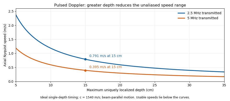
These are timing and sampling bounds, not a specification for a particular instrument. Pulse duration, scheduling and processing can lower the usable limit. Moving a spectral baseline changes the displayed signed interval but does not increase its total sampled-frequency width. Continuous-wave Doppler echocardiography avoids this pulse-rate restriction while sacrificing unique depth selection; high-pulse-rate acquisition instead accepts Doppler range ambiguity.^[ref] The acquisition choice determines which ambiguity remains.

At uniform sampling times $t_n=n/f_s$, adding an integer multiple of the sampling rate to a sinusoid's frequency changes its complex phase by an integer multiple of $2\pi n$. The samples therefore agree. Real cosines also identify the two signs of frequency, giving the displayed representative below the Nyquist frequency. A chosen nonzero sampling-time origin changes the equivalent phase, rather than the alias frequency.