The initial quantum state is a coherent state. Since and the state is normalized, its mean occupation number is . Each quantum harmonic oscillator energy eigenstate acquires the phase , soThe prefactor is a global phase and does not change an expectation value. Inverting the definitions of the annihilation operator and creation operator gives . If , thenFor a classical harmonic oscillator with amplitude , the conserved energy is . Setting gives exactly the same amplitude, . Thus these coherent-state oscillator expectation values follow the classical orbit.
The full quantum mean energy is nevertheless : the extra zero-point energy belongs to the nonzero position and momentum uncertainties required by the Heisenberg uncertainty relation, rather than to the motion of the packet centre. In particular, gives zero mean displacement but a finite ground-state width. A coherent state follows a classical mean trajectory while retaining finite position and momentum uncertainties.
Use the uncoupled angular momentum eigenstates and , with . For the Hamiltonian operator actually written in the paper, these are the energy eigenstates, withThe initial states are not all energy eigenstates of this operator. To find their energy populations, first perform the Clebsch-Gordan decomposition. The extremal states are and . Applying the total angular momentum lowering operator to the first givesSimilarly,The initial preparation is an equal incoherent mixture of the four coupled states. Each extremal state contributes population to its one energy eigenvalue, while each nonextremal state contributes and of its own population to the two displayed components. The resulting Zeeman splitting is thereforefor nonzero . The relative populations are in this order; the two zero-energy states each have population . These Zeeman populations from an unpolarized angular-momentum multiplet remain constant under subsequent evolution by the stated static Hamiltonian operator, although off-diagonal quantum coherence can evolve.
There is a distinct weak-field model in which a retained spin-orbit interaction keeps isolated and one projects the magnetic perturbation into that quartet. The Landé g-factor is then , giving four shifts with equal populations. That calculation requires the additional projection or dominant spin-orbit interaction; it is not diagonalization of the full magnetic Hamiltonian operator specified here, which also mixes the sector.
A confined ground state requires ; take so the trial wavefunction is normalizable. Its normalized form isThe Gaussian moment recurrence gives and . Also, integration by parts gives . The Rayleigh quotient for the quartic oscillator is consequentlyDifferentiation yields , so the unique minimum is at . Since the quotient diverges at both endpoints and , this is the global minimum in the trial family. The Rayleigh-Ritz variational principle givesFor the first excited energy eigenstate, choose the odd trial familyThe even confining potential has an even, nodeless ground state, by the nodeless theorem for a one-dimensional ground state. By the Sturm oscillation theorem, its first excited state is odd with one node. The proposed family has the same parity operator eigenvalue and one node, and is orthogonal to the exact ground state, not merely to its Gaussian trial approximation. Minimization in the odd linear subspace therefore bounds the first excited energy from above. For completeness, its Rayleigh quotient is , minimized at , giving . These are Gaussian variational bounds for a quartic oscillator.
If , there is no normalizable free particle ground state on the whole line, though the spectral infimum is zero. If , the Hamiltonian operator is not bounded below, so a ground-energy bound of the requested kind does not exist.
Start with the Schrödinger equation and differentiate the definition of the interaction picture state:The free Hamiltonian operator terms cancel because commutes with its own matrix exponential. ThereforeThis interaction picture transformation is exact.
Write and use the ordered spin basis . The free Hamiltonian operator is , soResolving the cosine into its two complex exponentials gives the exact upper off-diagonal factorwith the complex conjugate in the lower entry. Choose the field orientation with , as implicit in the printed near-resonance condition, and put . The rotating-wave approximation discards the terms at , retaining the slow terms at . The resulting interaction picture equations areThe factor contains from and from the cosine decomposition. This is a Driven two-level Rabi model, with signed on-resonance coupling and generalized Rabi angular frequency . Here the Rabi detuning uses the paper's convention, drive minus free frequency.
Small detuning alone is insufficient to derive the printed equations. One also requires , and an evolution time over which neglected terms stay small. At resonance this is the weak transverse-field regime . The supplied solution is thus an approximate solution for the linearly oscillating field, not an exact one at arbitrary drive strength. If , the other exponential is resonant and the physical positive resonance frequency is .
With , the Born rule applied to the supplied down-spin probability amplitude givesFor nonzero transverse field, the maxima occur atThe first maximum is reached at ; on resonance this is a Rabi pi pulse. The resonance envelope of a Rabi transition is a Lorentzian line shape, centred on under the orientation convention above. It has half its peak value at , so its full width at half maximum isIf resonance width is instead defined as the half-width, the ratio differs by a factor of two but has the same requested proportionality. The quality factor is large precisely in the regime where the rotating-wave approximation is justified. The envelope is obtained by choosing the best time separately at each drive frequency; a measurement at one fixed pulse duration has a different line profile.
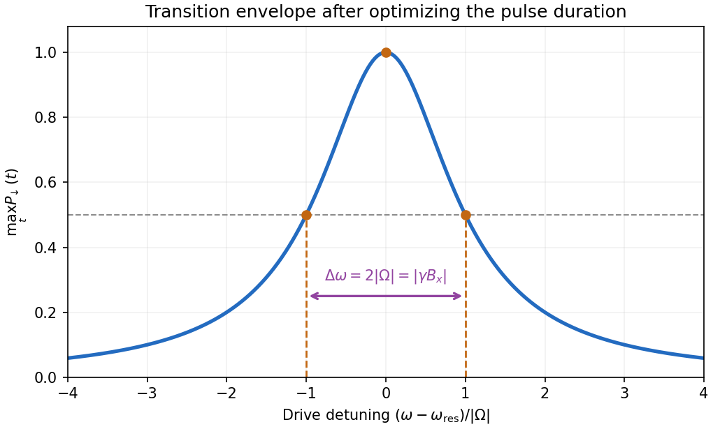
Maximum spin-flip probability versus drive detuning
. Original rotating-wave approximation envelope, with the two half-height detunings marked. The maximum is over interaction time independently at each drive frequency. Details.
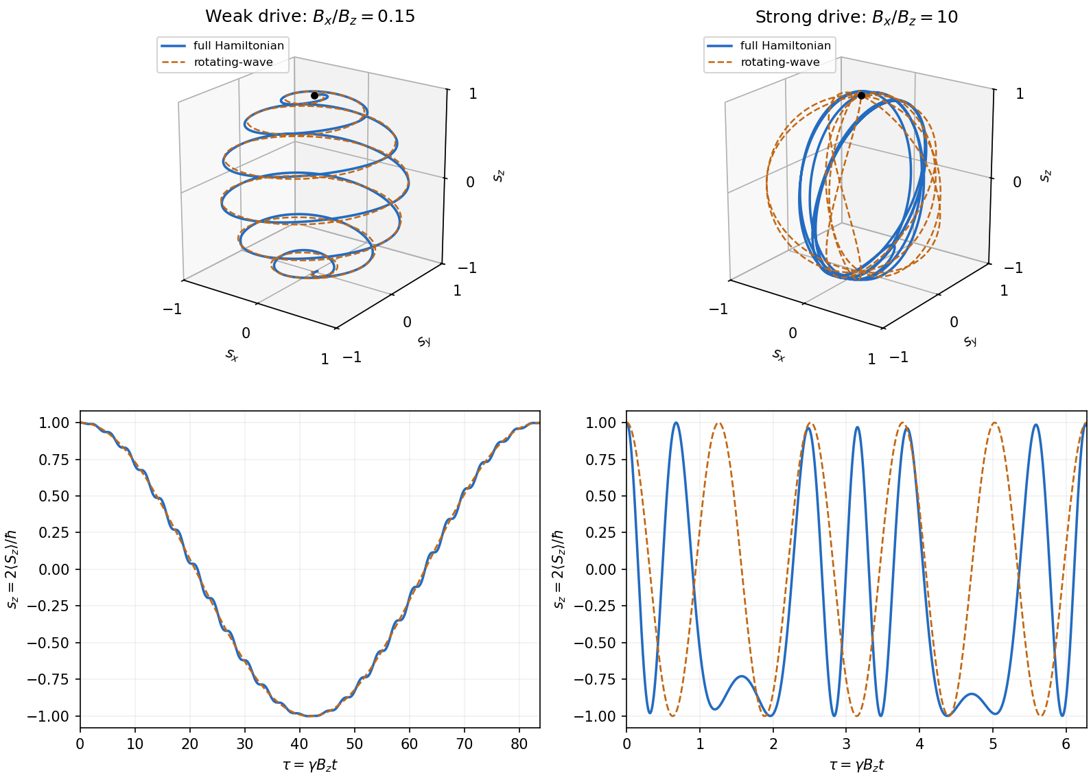
At resonance, retain the signed coupling . In the interaction picture, the given solution reduces to and . Returning to the Schrödinger picture givesFor a normalized spinor , the Pauli matrices give . Therefore the spin expectation value within the rotating-wave approximation isIts magnitude is : the Bloch vector stays on the unit sphere. In a frame rotating about at angular velocity , it makes a uniform rotation in the plane. For , this gives slow Rabi oscillations between the poles, accompanied by rapid laboratory Larmor precession about .
If the same formula is formally used for , it predicts fast meridional rotations whose plane turns slowly about . However, the original PDF really does ask for this opposite limit, and it lies outside the assumption used in part (b). That formal description is not a controlled prediction for the stated linearly driven Hamiltonian operator.
A valid strong-drive description starts from the exact equation for the Bloch vector :For times , neglecting the weak bias gives a controlled leading approximation, since the time integral of the omitted Hamiltonian operator has small norm. The remaining field has a fixed axis, so its generators commute at different times andAt the nominal resonance and on the early spin-rotation scale , this becomes . The initial rotation rate is consequently , twice the rate predicted by extrapolating the rotating-wave approximation. For longer times the exact differential equation must be retained. The following original calculation illustrates both regimes rather than asserting an exact strong-drive Rabi formula.

The components of the momentum operator do not generally commute with a position-dependent magnetic vector potential. Expanding minimal coupling with the ordering intact givesActing on a wavefunction shows that . In the Coulomb gauge the divergence vanishes, so the two cross terms agree. Discarding the quadratic term in the weak radiation amplitude givesThe equality of the two operator orderings follows from the gauge condition, not from treating and as commuting numbers component by component.
For the requested oscillator response, treat as the fixed transverse position of a one-dimensional quantum harmonic oscillator along , and put . The supplied radiation is transverse and already satisfies the Coulomb gauge. Its perturbation isThe annihilation operator and creation operator giveThus the only first-order transition out of the ground state is to . More generally, the oscillator electric-dipole selection rule is . This is a rule for matrix elements; exact energy conservation is replaced by a finite-time resonance profile during a switched finite-duration interaction.
To display both the resonant and nonresonant terms without spurious singularities, defineThe interaction picture coefficient in the given expansion is thenThe full Schrödinger picture coefficient of is , while that of is at this order. The normalization changes only at order . In particular, at the first term is , finite for every finite time, and the perturbative result requires .
The fixed- interpretation is needed for the displayed target formulae. If were instead a three-dimensional kinetic operator with no transverse confinement, that model would have no normalizable transverse ground state, and would transfer transverse momentum . A treatment of that different model needs specified transverse states and recoil energies; they are absent from the question. The following parts use the intended localized-oscillator response.
The only relevant position matrix element is . To first order in the radiation amplitude, the two ground–excited-state cross terms giveMultiplying by the charge gives the induced electric dipole moment. Since , the coefficient derived in part (b) yieldsat linear order. Taking the complex conjugate inside the real part of the second term changes it to minus the same term with and reversed frequency signs. ThusThe terms at are switch-on transients, while those at describe the driven response. Both are needed to make . The expression is understood by continuity at ; the first quotient then tends to , producing resonant secular growth rather than an infinite dipole at a finite time.
There is also an initial-velocity check on this harmonic-oscillator dipole response to switched radiation. The formula gives . Because the magnetic vector potential jumps at zero time, its time derivative contains an impulsive electric field. Equivalently, the mechanical velocity is , whose initial mean is . The transient therefore implements the specified switch-on correctly.
For , isolate the terms proportional to in the previous answer. Their coefficient isHence the driven electric dipole moment component isFor , away from the instantaneous switch, the radiation electric field isThus the dynamic electric polarizability isBelow resonance the driven electric dipole moment is in phase with the electric field; above resonance its sign reverses. The same susceptibility follows from the classical Lorentz oscillator model without damping. At exact resonance the separation into bounded driven and transient terms fails: their apparent poles combine into the finite-time secular term identified in part (c). Without damping there is no bounded steady resonant response, and the first-order state expansion eventually ceases to apply.
Inside the infinite square well, the orbital and spin operators act on different factors of the tensor product. Write . The identityshows that the exchange interaction commutes with and . The sum of the one-particle kinetic energies also commutes with them and with particle exchange. Thus one may use orbital quantum numbers together with the total-spin sector and projection , with physical .
For identical spin one-half particles the Pauli exclusion principle further restricts the states. The spin-one-half singlet state is antisymmetric in spin and must multiply a symmetric spatial wavefunction; a spin-one-half triplet state must multiply an antisymmetric spatial wavefunction. Thus label unordered orbital occupations in symmetry-adapted states, not arbitrary ordered product states. This gives the labels , with the paper's last label expressed in units of .
LetThe normalized orbital energy eigenstates vanish outside the well and have one-particle energies . Define the normalized symmetric and antisymmetric combinations for byThe normalized spin functions are the singlet state and the triplet states , , . Their exchange energies are respectively and .
For , the three lowest distinct energy levels of the exchange-coupled spin-one-half particles in an infinite square well areThe spatially doubly occupied orbital can only occur with the singlet state. The next orbital sum is , where either exchange symmetry is possible. The next unused sum is , well separated under the small-coupling assumption. The paper's inequality is equivalent, up to a numerical factor, to ; the factor in is essential because the spin operators carry units of angular momentum.
The sign of is not explicitly specified. The table assumes the usual intended positive coupling in the displayed minus-sign convention. For with , the same three sets of eigenfunctions occur, but the two rows at exchange order. At those rows merge into a single energy level of multiplicity four; if three distinct energies are requested exactly at that point, the third is with the single state .
Each one-particle energy eigenstate has definite parity about the centre of the well, so . Consequently, a doubly occupied orbital has . For distinct orbitals, the two off-diagonal exchange terms instead survive:The position matrix elements in a symmetric infinite square well, with the present width , giveThe sign of depends on the orbital phase convention, while does not. The perturbation acts only on the spatial part and cannot mix orthogonal singlet states and triplet states. Within a triplet it is proportional to the identity on the spin factor. Thus first-order nondegenerate perturbation theory, with this trivial diagonal treatment of spin degeneracy, gives the shifts corresponding to the three rows in part (b):These formulae also apply for , with the reordered levels described above. At , they resolve the fourfold level into a shifted triplet and singlet. The next doubly occupied orbital still has zero first-order shift. The perturbative requirement is for mixing with remote orbital states; the spin-independent perturbation does not require division by the small singlet–triplet gap.
For distinguishable particles, the ordered spatial products are independent states, and neither singlet states nor triplet states are excluded from any orbital occupation. The unperturbed energy eigenvalues areFor , the three lowest distinct energy levels arewhere . The first two levels do have zero first-order correction, since their spatial expectation value factorizes as .
The last instruction in the original PDF is false for the third level. Although every diagonal product-state matrix element vanishes, the two orbital states have degenerate energy levels. Degenerate perturbation theory requires diagonalizing the perturbation within their span. For each , its matrix in the ordered basis isThe eigenfunctions are , withThus the sixfold unperturbed level splits into two triplets. Its average shift is zero, and the diagonal expectation in an individual ordered product state is zero, but neither fact makes all its energy eigenvalue corrections zero. This is the degenerate orbital exchange splitting from a product perturbation; distinguishability allows both combinations rather than removing their coupling.
For negative , the lowest two rows exchange order and the third unperturbed level is instead the twofold singlet orbital pair at . It splits into with the same shifts , each nondegenerate. At , the three lowest distinct unperturbed energies are , with multiplicities . The first and third have zero first-order shift; the middle splits by , each fourfold. The printed zero-shift assertion therefore fails also in the zero-exchange limit.
Articles by others on the same topic
There are currently no matching articles.