Past exam of the advanced quantum physics course of the University of Cambridge / 2022 / Section B

Let the electric charge be $q=-e$, where $e>0$ is the elementary charge. Minimal coupling to a tangential magnetic vector potential givesA constant tangential magnetic vector potential is an available gauge on the ring, so $a=q{A}_x$. By Stokes theorem, its circulation is the oriented magnetic fluxThe orientation matters here. In the original diagram, increasing $x$ goes anticlockwise, whose associated positive normal points out of the page, whereas the indicated positive magnetic flux $\Phi$ points into the page. Hence ${\Phi }_C=-\Phi$ for that diagram, and its convention gives $\boxed{aL=e\Phi }$. If instead $\Phi$ is defined with the normal associated to $+x$, the relation is $aL=-e\Phi$.

There is no requirement that the magnetic field be nonzero on the ring: it can be confined to a solenoid inside it. The nonzero circulation of the magnetic vector potential still affects the Electron through the Aharonov-Bohm effect.

Define a transformed wavefunction byIndeed, writing $\psi =e^{iax/\hslash }\tilde{\psi }$ givesThis is the electromagnetic gauge transformation generated by $\chi (x)=-A_{x}x$: $A_x^{\prime }=A_x+{\partial }_x\chi =0$ and ${\psi }^{\prime }=e^{iq\chi /\hslash }\psi$. The transformed Hamiltonian operator is consequently $p^2/(2m)$, but the original periodic boundary condition becomes the twisted boundary conditionFor the domain of the self-adjoint kinetic Hamiltonian operator, the derivative has the same twist, ${\tilde{\psi }}^{\prime }(x+L)=e^{-iaL/\hslash }{\tilde{\psi }}^{\prime }(x)$. Thus the magnetic flux has moved into the boundary condition. The transformation is a single-valued gauge on periodic representatives only when $aL/\hslash$ is an integer multiple of $2\pi$; otherwise it is understood on the cut interval with the displayed identification of its endpoints.

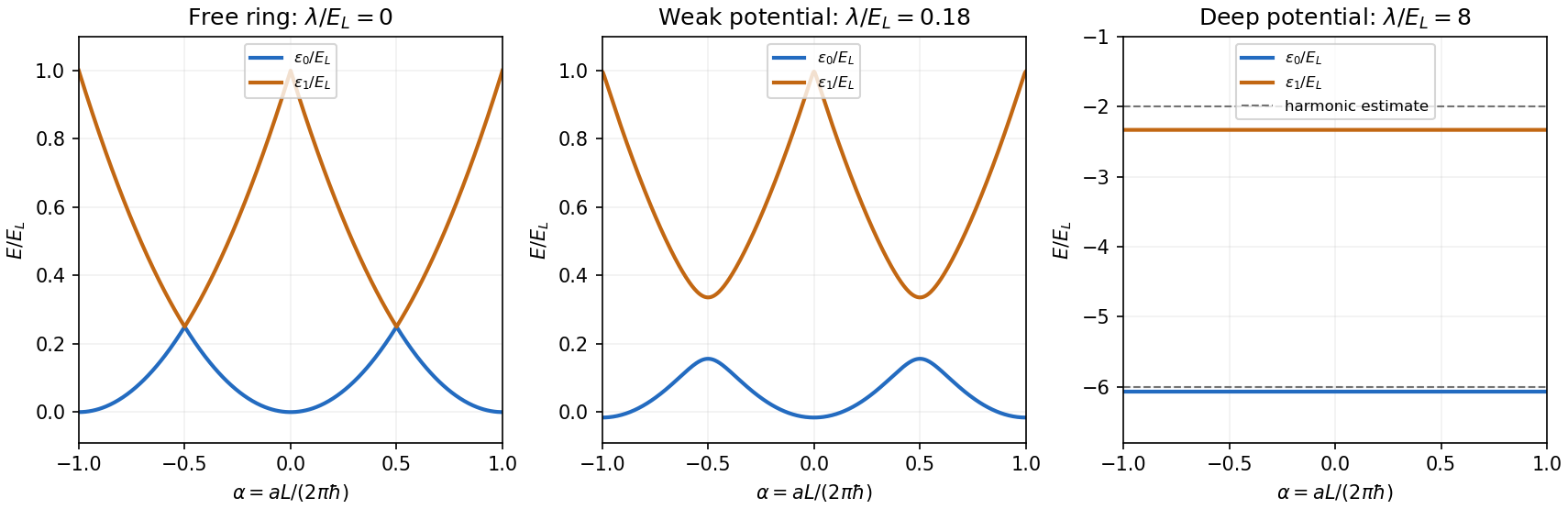
For the magnetic flux spectrum of a quantum ring, the periodic boundary condition permits the normalized plane waves $L^{-1/2}{e}^{2\pi inx/L}$, with $n\in \mathbb{Z}$. Their energy eigenvalues areShifting $\alpha$ by an integer relabels $n$, so the ordered energy levels have period one in $\alpha$, or $2\pi \hslash /L$ in $a$. For $-1/2\le \alpha \le 1/2$, the lowest two areextended periodically. The lowest branches cross at every half-integer $\alpha$, with energy $E_L/4$. At integer $\alpha$, the first excited energy level has multiplicity two. The corresponding magnetic flux period is the electron magnetic flux quantum $h/e$.

In the normalized plane wave basis, the only nonzero potential matrix elements areThus a useful small parameter is $|\lambda |/E_L\ll 1$, which suppresses admixture of well-separated energy levels. First-order nondegenerate perturbation theory further requires $|\lambda |/2\ll |E_n-E_{n\pm 1}|$ for the coupled states. This latter condition fails near a half-integer $\alpha$ even for very small $\lambda$; there one must use degenerate perturbation theory in the nearly degenerate pair. Smallness is measured against the gaps to the other states, not the vanishing gap inside this pair.

Near $\alpha =1/2$, keep $n=0,1$. The resulting Hamiltonian operator matrix and its eigenvalues areIn particular,For positive $\lambda$, the lower quantum state at the crossing is the symmetric combination of $n=0,1$, and the upper state is the antisymmetric combination. A negative $\lambda$ exchanges these combinations but leaves the ordered energy eigenvalues unchanged.

This cosine-potential gap in a quantum ring appears in the middle panel above: each lowest-branch crossing opens into an avoided crossing of gap $|\lambda |$ to first order. Away from these crossings, the diagonal matrix elements vanish, so the leading shifts are second order. At integer $\alpha$, the two first-excited plane waves differ by two units of $n$ and therefore have no first-order coupling; their smaller splitting begins at second order. The numerical plot includes that splitting.

Put $\Lambda =|\lambda |\gg E_L$. Changing the sign of $\lambda$ translates the potential by $L/2$ without changing its energy eigenvalues, so take a minimum at $x=0$ and expand there. The parabolic approximation givesThe low-lying wavefunctions are localized well inside one period. A local gauge transformation removes $a$ from their quantum harmonic oscillator equation, givingConsequently,The sketch consists of two nearly horizontal branches, separated by this gap, as in the right panel above. The parabolic approximation makes them completely independent of magnetic flux; in the actual ring they retain exponentially small periodic dependence through quantum tunnelling around the ring. Corrections from the nonquadratic part of the potential shift the mean energies and gap by relative order $\sqrt{E_L/\Lambda }$, whereas the tunnelling dependence is smaller than every power of that parameter.

The unperturbed infinite square well is invariant under the parity operator. Its one-dimensional energy eigenvalues are nondegenerate, so each energy eigenstate has definite parity. Its position expectation value therefore vanishes: $|{\varphi }_n(x){|}^2$ is even, while $x$ is odd. The first-order nondegenerate perturbation theory correction is consequentlyThe electric field does mix opposite-parity quantum states, and second-order nondegenerate perturbation theory contains two factors of $eEx$. Its leading contribution is thus proportional to $E^2$: this is a quadratic Stark effect. More generally, applying the parity operator changes $H(E)$ into $H(-E)$, so their corresponding energy eigenvalues agree. An analytic expansion about zero electric field contains only even powers of $E$. We assume $e|E|a$ is small compared with the unperturbed excitation scale.

Use zero-based labels to agree with ${\varphi }_0$ in the later parts. The normalized infinite square well energy eigenstates and energy eigenvalues areThe position matrix elements in a symmetric infinite square well, obtained by integrating the product of the two wavefunctions against $x$, areThe integral in the question uses positive integer labels; replacing them by $k+1,n+1$ is essential here. Only opposite-parity states, $k+n$ odd, contribute, as also follows from the parity operator selection rule.

Second-order nondegenerate perturbation theory now gives the requested infinite sum:In fully explicit form this isThe symbol $m$ here denotes the electron mass, not a summation index. For the ground state $n=0$, every denominator in the first form is negative, so the ground energy level moves downward. For excited states, contributions from lower and higher energy levels have opposite signs.

The electron's electric dipole moment is $\mathbf{d}=-e⟨x⟩\hat{\mathbf{x}}$. It vanishes in the unperturbed ground energy eigenstate. The first correction to the wavefunction is linear in the electric field and has the opposite parity; its interference with the unperturbed state therefore gives a nonzero position expectation value of first order.

In detail, the normalized ground quantum state, to the order needed, isThe normalization correction starts at second order and does not affect the linear term below. The two cross terms giveThe absence of an $E^2$ term follows from the parity operator: $⟨x⟩$ changes sign under field reversal. Comparing with the second-order nondegenerate perturbation theory energy sum yieldsThus the induced electric dipole moment points along the electric field, with positive electric polarizability. The induced dipole moment and quadratic energy shift obey $\delta {ϵ}_0^{(2)}=-{\alpha }_{\mathrm{pol}}{E}^2/2$. This factor of one half accounts for the energy needed to induce the dipole. As a check, the Hellmann–Feynman theorem gives $d_x=-\partial {ϵ}_0/\partial E$, with the same result.

Normalize the trial quantum state as $(|{\varphi }_0⟩+c|{\varphi }_1⟩)/\sqrt{1+c^2}$. With the phases used above, the off-diagonal position matrix element is $x_{01}=-32a/(9{\pi }^2)$. DefineThe diagonal perturbation matrix elements vanish by parity, so the Rayleigh quotient isThe stationarity equation is $W+\Delta c-W{c}^2=0$. The minimum continuously connected to the unperturbed ground energy eigenstate hasEquivalently, diagonalize the Hamiltonian operator matrix in this two-dimensional trial space. Its lower eigenvalue isThereforeThis retains exactly the $k=1$ term of the full ground-state second-order nondegenerate perturbation theory sum. Every omitted term is negative, so the full quadratic correction is more negative than this restricted one. This is consistent with the Rayleigh-Ritz variational principle: minimizing over a two-state subspace gives an upper bound on the exact ground energy. The bound applies to the unexpanded two-state minimum; a truncated series is to be compared order by order.

For this spin-boson model, take $H_0=H_1+H_2$. Since $[H_0,{\sigma }_z]=0$, the interaction picture observable isThe normalized vectors $|{\varphi }_{\uparrow }⟩$ and $|{\varphi }_{\downarrow }⟩$ belong to different eigenspaces of the Hermitian operator ${\sigma }_z$, and are therefore orthogonal. This remains true even though each vector includes the oscillator degrees of freedom. Hence all cross terms in the expectation value vanish, while the diagonal terms have eigenvalues $+1$ and $-1$:Normalization also gives $|c_{\uparrow \sigma }{|}^2+|c_{\downarrow \sigma }{|}^2=1$, so these are the probabilities of the two spin outcomes.

The orthogonal projection onto the full spin-$\eta$ subspace isHere the identity acts on all oscillator states. The finite-time scattering operator $S(t)$ in the question is the interaction picture time-evolution operator, so $|{\psi }_{\sigma }^I(t)⟩=S(t)|\sigma ,\{n\}⟩$. Projecting its two orthogonal spin components yieldsExpand the right-hand side in the orthonormal basis $|\eta ,\{n^{\prime }\}⟩$. Taking its squared norm, and using the normalization of $|{\varphi }_{\eta }⟩$, givesThus one sums probabilities over unobserved final oscillator states, not their probability amplitudes. Unitarity of $S(t)$ makes the sum over both $\eta$ equal to one.

The Pauli matrix ${\sigma }_x$ flips the spin with unit matrix element. A nonzero oscillator matrix element changes exactly one occupation number, through a creation operator or an annihilation operator:For a spin flip, the spin energy change divided by $\hslash$ is $-s_{\sigma }\Omega$. Thus creation and annihilation in mode $j$ have total frequency changes ${\omega }_j-s_{\sigma }\Omega$ and $-{\omega }_j-s_{\sigma }\Omega$, respectively. Distinct modes or different occupation changes lead to orthogonal final quantum states, so their probabilities add. Fermi's golden rule consequently givesThe Dirac delta function is even, accounting for the sign in the annihilation term. Since all ${\omega }_j,\Omega >0$, an initially up spin can only emit an oscillator quantum, while an initially down spin can only absorb one. Writing the oscillator density of states per unit angular frequency as $g(\omega )={\sum }_j\delta (\omega -{\omega }_j)$, the continuum limit givesThe $+1$ permits emission even from the oscillator vacuum; absorption requires a quantum already present. The notation $n_{\Omega }$ assumes a common or smoothly specified occupation at the resonant frequency. If several resonant modes have different occupations, it denotes their density of states weighted mean, so that $g(\Omega )n_{\Omega }={\sum }_j{n}_j\delta (\Omega -{\omega }_j)$ after continuum smoothing. This is the golden-rule relaxation of a spin coupled to an oscillator bath.

In first-order time-dependent perturbation theory, the resonant time factor before taking the Fermi's golden rule limit isIts central frequency width is of order $1/t$, and its total area is $2\pi t$. To replace it by $2\pi t\delta (\nu )$, the oscillator density of states and relevant occupations must be approximately constant over that width. Thus $t\Delta \omega \gg 1$. At the same time, the perturbative flip probability must remain much smaller than one.

Define ${\Gamma }_0=2\pi {\lambda }^{2}g(\Omega )/{\hslash }^2$, so the two flip rates are ${\Gamma }_0(n_{\Omega }+1)$ and ${\Gamma }_0{n}_{\Omega }$. A sufficient common time window for both initial spins isFor a specified initial spin, the upper condition is simply its own flip rate times $t\ll 1$. Such a window requires weak enough coupling. The continuum approximation also presumes times shorter than recurrences from a resolved finite oscillator spectrum, and long enough to resolve the positive-frequency resonance from its nonresonant counterpart.

The thermal oscillator occupation is the Bose-Einstein distribution. With the rate notation ${\Gamma }_{\eta \sigma }$ for a transition from $\sigma$ to $\eta$, the master equation for the up population isAt thermal equilibrium, assuming ${\Gamma }_0>0$, vanishing time derivative is detailed balance between the two spin states. HenceorTogether with normalization, this gives $p_{\uparrow }=1/(1+e^{\beta \hslash \Omega })$ and $p_{\downarrow }=e^{\beta \hslash \Omega }/(1+e^{\beta \hslash \Omega })$, the Boltzmann distribution for the energy eigenvalues $\pm \hslash \Omega /2$. At zero temperature, absorption vanishes and emission relaxes the spin into its down ground state.

The nonzero-rate condition is necessary: if $\lambda =0$ or $g(\Omega )=0$, both rates vanish, so every initial pair of populations is stationary within this approximation. In that case stationarity alone cannot imply a thermal distribution. The equilibrium conclusion therefore presumes coupling to resonant oscillator modes.