Source release: Oxford examination archive release thread. The four-page scan is from pages 434–437 of the released Part C bundle. The cover identifies paper C6.3b, formal codes
DMAC 2B68 and DMCO 2B68, and Thursday 9 June 2011.Answer availability checked on 28 October 2026: bounded searches of official Oxford sources by year, course name, paper label and formal code found no advertisement of complete or selected-part answers for this exact paper. The departmental examination overview does not establish solution availability for this 2011 paper.
Put , so the interior angle at the th polygon vertex is . A conformal map straightens that corner by a power: locally,This follows by composing with the power that maps the corner to a half-plane and using Schwarz reflection along its straight edges. The reflected map has a nonzero first derivative in the straightened coordinates.
For an upper-half-plane branch of the complex logarithm, defineAlong each open interval of the real axis, has constant argument. Crossing from left to right decreases from to zero, so the argument of increases by . This is exactly the exterior turning angle of the polygon boundary. Thus has one constant boundary argument on all the intervals. The corner asymptotics remove its apparent singularity at each prevertex.
For a bounded polygon, the sum of exterior angles gives . Since every vertex has a finite prevertex, infinity maps to an ordinary point of an edge. In the local coordinate , Schwarz reflection gives with . Hence has a finite nonzero limit at infinity. After multiplication by one unit complex number, its boundary values are real. Reflecting across the real axis extends it to an entire function, including each removed prevertex, and it is bounded at infinity. Liouville's theorem makes it constant. Therefore the Schwarz-Christoffel formula isIntegration introduces one further additive constant.
The Möbius transformations preserving the upper half-plane have three real parameters:with common nonzero scaling irrelevant. They can send any cyclically ordered triple of boundary points to another such triple. Consequently three prevertices may be fixed independently; the other are constrained by the polygon's shape, through its side-length ratios. The constants of integration and multiplication account for translation, rotation and scale of the image, rather than further prevertex freedom.
If the last prevertex is infinity, use as its local coordinate. Its factor is absorbed into the overall normalization, leavingFor a finite image vertex at infinity's preimage, this has asymptotic order , because is of order . Thus the omitted factor is not evaluated by substituting infinity into the finite product; its angle is encoded by the behavior at infinity.
The two approaches to the slit base are distinct boundary points, each with interior angle , whereas the slit tip has interior angle . Their exponents in the Schwarz-Christoffel formula are therefore , and . Write and takeon the upper half-plane, with the branch normalized by at infinity. The derivative has the formOn , the upper boundary value is . Both endpoints of this interval map to the slit base, soThe odd term integrates to zero, and ; hence . Now , so . The endpoint values force , and the tip value, using as a boundary limit, forces . ThusThe branch is important: on its boundary value is positive real, on negative real, and on positive imaginary. The intervals and traverse the two sides of the slit, meeting at its tip.
The map is injective in the upper half-plane: equal images imply , and the alternative cannot put both points in that half-plane. Its derivative has no interior zero. The image has positive imaginary part, by continuity of the branch and the fact that an interior real image would require to be nonnegative real, which is impossible for . Conversely, a point in the upper half-plane outside the slit gives a unique upper-half-plane root of . A point with gives only real roots or zero and is excluded. These observations verify that the image is exactly the required slit domain, rather than just matching its boundary.
The imaginary part of the complex potential of a two-dimensional potential flow is the stream function. Its constant values on the wall and the free boundary make the potential domain the horizontal stripThe lower edge is the rigid wall, with at . The upstream end has , and the downstream end has . The upper edge is the free streamline. Thus and are the negative and positive portions of the real axis, respectively.
Write for the complex velocity. Downstream . Upstream the fluid moves towards the corner along a wall of inclination , so its physical velocity has argument and its complex velocity has argument . Along each straight wall the velocity direction is fixed. At the corner the fluid angle is , giving local behavior and hence : is a stagnation point. On the free streamline, the speed is one, so .
The corresponding simple-jet hodograph plane is therefore the circular sectorThe radius at argument represents , the positive real radius represents , and the unit-circle arc represents the free boundary. The upstream and downstream ends are and one, respectively; the corner is the sector's origin.
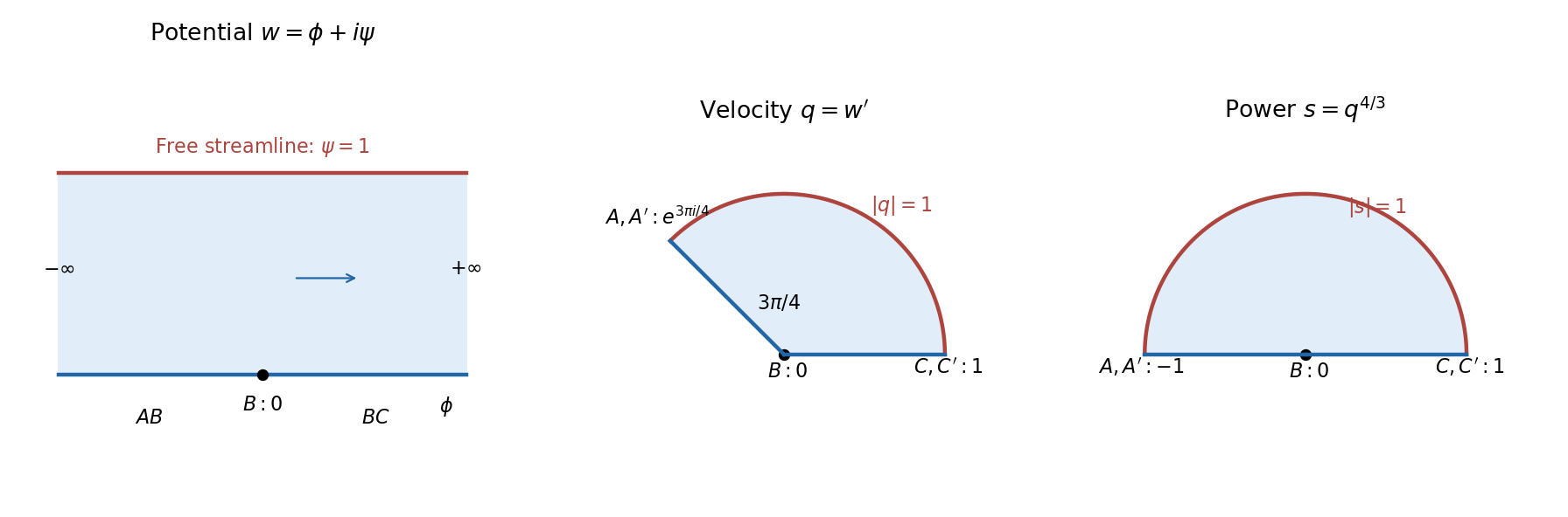
The complex potential of a two-dimensional potential flow strip and hodograph plane, with an intermediate power map
. Details. 
Starting from the hodograph plane, take the complex powerIt takes the velocity sector bijectively to the upper half of the unit disk. The boundary points representing the upstream end, the corner and the downstream end become , zero and one. Next use the Möbius transformationThe diameter maps to the negative real axis, while for on the upper semicircle,which is on the negative imaginary axis. The interior maps to the third quadrant. Squaring therefore gives a conformal bijection from that quadrant to the upper half-plane:The upstream end, corner and downstream end map to zero, one and infinity, respectively. The two walls map to the positive real axis, and the free boundary maps to the negative real axis.
Independently, the exponential function takes the potential strip to the same upper half-plane with the same boundary correspondence. The strip height fixes the coefficient , and the normalization fixes the remaining positive multiplicative constant in to one. ConsequentlyOne can make the branches explicit. In the strip, lies in the first quadrant, whereas . Thuswith the power taking arguments in to . It gives upstream, downstream, and at , verifying both the branch choice and the velocity normalization.
Let be the inverse conformal map. With real and nonzero, the function is harmonic away from the source, vanishes on the moving boundary, and has the required logarithmic singularity. Indeed with , so near the origin. Subtracting this candidate from the physical velocity potential leaves a bounded harmonic function near the source. Its singularity is removable, and the difference has zero boundary values. The maximum principle for harmonic functions makes it identically zero. ThereforeOnly the real part is needed, so the multivalued imaginary part of the logarithm causes no ambiguity in .
Differentiate while holding the physical point fixed:Also the local analytic complex potential of a two-dimensional potential flow has derivativeThe distinction between differentiating at fixed and fixed is essential because the boundary map depends on time. Substituting into the boundary evolution law and multiplying by givesTaking the conjugate inside a real part leaves it unchanged, so the desired conformal map equation for planar Darcy growth isAs a normalization check, parameterize the boundary by . Its outward normal vector times arclength is , so its area growth rate is , exactly the specified source flux. For an expanding circular map , the equation reduces to .
Orient the contour and call its left-hand side the plus side. At a smooth interior point , take a local arclength parameter with . The Cauchy principal value means the symmetric deletion limitThe two local pieces are deleted with the same arclength cutoff. For a sufficiently smooth regular contour, an equal-radius deletion about gives the same limit. The point is assumed to be away from endpoints and self-intersections.
To derive the Sokhotski–Plemelj formula, split the contour into a short smooth arc through and its complement. The complementary integral has the same limit from both sides. On the short arc subtract from the numerator. Because is holomorphic nearby, extends continuously as approaches ; this part also has the same limit from either side. The remaining local term is . Straightening the oriented tangent shows its extra contribution is from the left and from the right: on a real segment this is the direct limit of . Dividing by yieldsIn particular the jump is , while the sum is the principal-value integral divided by . Smooth densities on a real interval satisfy the same formulas at every interior point, by the identical subtraction step with a Hölder-continuous remainder.
Now put . On the interval, the sign reversal of the auxiliary boundary values givesThus the required Cauchy transform density isWhenever this density is integrable at the endpoints, taking constructs a function with the required jump. Multiplication back gives . The jump of the constructed isTo conclude that this jump solves the final singular equation, one must additionally justify . This reconstruction requires endpoint and infinity conditions; the sign reversal of alone does not ensure it. Here is a complete valid normalization. LetThe branch is holomorphic off , with and . If extends smoothly to , the density vanishes like a square root at each endpoint. Its Cauchy transform is bounded at the endpoints and is at infinity. Therefore is at most inverse-square-root singular at each endpoint and is at infinity. Its jump is integrable.
For Cauchy reconstruction from a jump across a finite interval, apply the Cauchy integral formula to on a large slit contour, and shrink its banks to . The large circle contributes zero in the limit; each small endpoint circle contributes and also vanishes. The two banks give the jump , proving . The sum part of the Sokhotski–Plemelj formula now givesThis proves the intended finite Hilbert transform inversion with admissible endpoint behavior. Adding a multiple of to gives a homogeneous solution; equivalently one can add a constant multiple of to , whose boundary sum is zero.
The omitted normalization is a real limitation of the printed claim. To see it explicitly, choose instead and . This auxiliary function satisfies all the stated holomorphicity, nonvanishing and sign-reversal requirements. ButThe displayed integral identity follows from and its continuation from real . Hence the proposed jump formula gives , which does not solve the equation with . The failure is the nonzero constant at infinity: . Thus the final implication is valid with suitable endpoint and decay conditions, but is false for an unrestricted auxiliary function as printed. The valid reciprocal-square-root normalization above supplies an actual solution for smooth up to the two endpoints.
In the Laplace integral method for a differential equation, differentiate the integral three times with respect to , and replace by . Integration by parts givesThus the weight equation for this construction and its boundary condition arewhich giveThese are the conditions obtained by eliminating the transformed interior term and the endpoint term separately. As usual for this method, differentiation and integration by parts need convergence assumptions; the contours constructed next make every such step valid locally uniformly for all complex . A literal necessity claim for arbitrary weights and contours would additionally require uniqueness of the chosen representation by a Laplace integral; a null weight in a contour Laplace representation can otherwise be added without changing the solution.
LetThe quartic decay sectors for a contour integral contain the four rays . Along each ray, the quartic term is . For , choose to travel from infinity on ray to zero, and then from zero to infinity on ray . Set and defineOn any compact set of values, the integrand and each of its derivatives are bounded by a constant times for some . These bounds are integrable at infinity, so differentiation under the integral sign is justified and the functions are entire. The endpoint term vanishes at both infinite ends. There is no extra term at zero because the two pieces join with the same integrand value and opposite endpoint orientations. Therefore all three functions solve the differential equation.
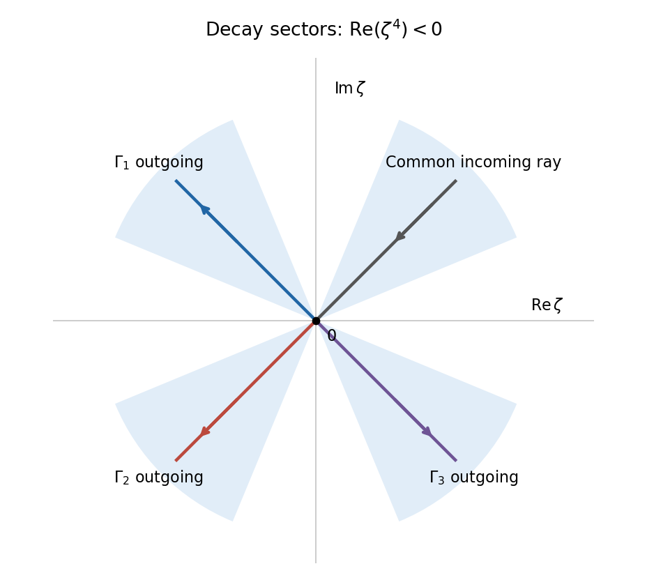
Three independent Laplace integral contours joining rays in quartic decay sectors
. Details. 
To prove independence, evaluate their first three initial data. For ,If , these initial data give for . Define . ThenThe coefficient matrix is a Vandermonde matrix at four distinct fourth roots of , and hence is invertible. All vanish. There is also a concrete reason for the earlier qualification about necessity. Deform the incoming ray of to angle and its outgoing ray to angle , within their respective quartic decay sectors. The quartic integral is unchanged and remains nonzero. On this deformed contour, the extra entire weight contributes zero for every : throughout the closing wedge, , so the large closing arc tends to zero and the Cauchy integral theorem gives a zero integral. Thus represents the same entire solution and has vanishing endpoint terms, although it does not satisfy . The canonical weight equation is the standard sufficient construction, rather than an unconditional uniqueness assertion about contour representations.
Thus the three contours give linearly independent nonzero solutions, and they form a fundamental system of solutions for this third-order linear equation. This proves independence directly instead of inferring it merely from the presence of three different contours.
Write , and . In a common convergence strip, two integrations by parts on each half-line giveThe boundary terms at infinity vanish by exponential decay; the ordinary differential equations also give decay of the required first derivatives. Substituting the two equations for yieldsContinuity makes the terms cancel on addition, while the unit derivative jump givesMultiply by and factor the quadratics. Since , their sum is nonzero, and partial fractions giveThis is the Wiener-Hopf equation for the two half-line Fourier transforms. The plus and minus subscripts refer to support in physical space; their holomorphic domains in transform space are determined next.
Let . On , the modulus of the Fourier factor is , so the given decay bound makes converge absolutely when . On , write ; the bound becomes , so converges absolutely when . Uniform domination on compact subsets permits differentiation with respect to , provingThus the half-planes guaranteed directly by the given common decay bound have and , and the equation holds on their overlapThis is a statement about the domains guaranteed by that bound, not necessarily their largest possible domains. The exact solution below decays at different rates on the two half-lines and gives the sharper convergence half-planes and , with maximal common strip .
The constant-coefficient equations and decay imply that only the modes on the positive half-line and on the negative half-line can occur; the opposite modes grow. Continuity and the nonzero derivative jump then imply nonzero amplitudes, so any common decay exponent satisfies . In particular lies below the plus holomorphic half-plane, and lies outside the minus half-plane. This locates the poles needed for the transform calculation, without yet computing the amplitudes.
Rearrange the equation from part (i) asThe left side is holomorphic in the plus half-plane, and the right side in the minus half-plane. Their equality on the overlap glues them into one entire function. The assumed decay of , together with the rational factors tending to one and the subtracted fractions tending to zero, makes this entire function tend to zero at infinity. It is therefore identically zero by Liouville's theorem. This is the additive splitting step of the Wiener-Hopf method. Solving the two zero identities givesTheir apparent cancellation formulas extend holomorphically wherever a cancelled factor vanishes; the only actual poles are at and .
With the Fourier convention in use, inversion has factor and normalization . For , close the contour in the lower half-plane clockwise, collecting the pole at . For , close in the upper half-plane counterclockwise, collecting the pole at . The residue theorem givesEquivalently, each displayed transform follows immediately by integrating the corresponding decaying exponential on its half-line, so Fourier uniqueness gives the same inversion without a contour estimate. Both values at zero are , and the derivative jump is , directly checking the interface conditions.
The moduli are a nonzero constant times for and for . Hence the largest common exponential decay rate isStrictly, the stated big- bound is also true for every smaller positive ; it does not specify a unique exponent unless the sharp rate is intended. The two transform convergence half-planes are exactly the sharper domains stated in part (ii), and the poles on their boundaries prevent extending either half-line integral domain any farther.
Articles by others on the same topic
There are currently no matching articles.