Original solutions to both sections and all six questions of the Approximation Theory and Finite Element Methods paper sat on 10 June 2010. Source: released Mathematics papers,
Part C 2007 11.pdf. Question 1 gives the sharp bound for the printed functional; question 4 distinguishes the printed normal condition from the conormal condition needed for the requested symmetric variational construction. Statements are not reproduced.Direct evaluation gives and . Hence the linear functional vanishes on every polynomial of degree at most two and is nonzero on every genuine cubic polynomial.
The Peano kernel theorem with order three gives , whereThe first term comes from differentiating at . On the integration interval this simplifies toIn particular . Its L1 norm is , so the sharp bound isThe printed constant is false for the printed functional. The cubic has but , and it attains the corrected bound. This is an exact Peano kernel norm calculation, not an error from numerical quadrature.
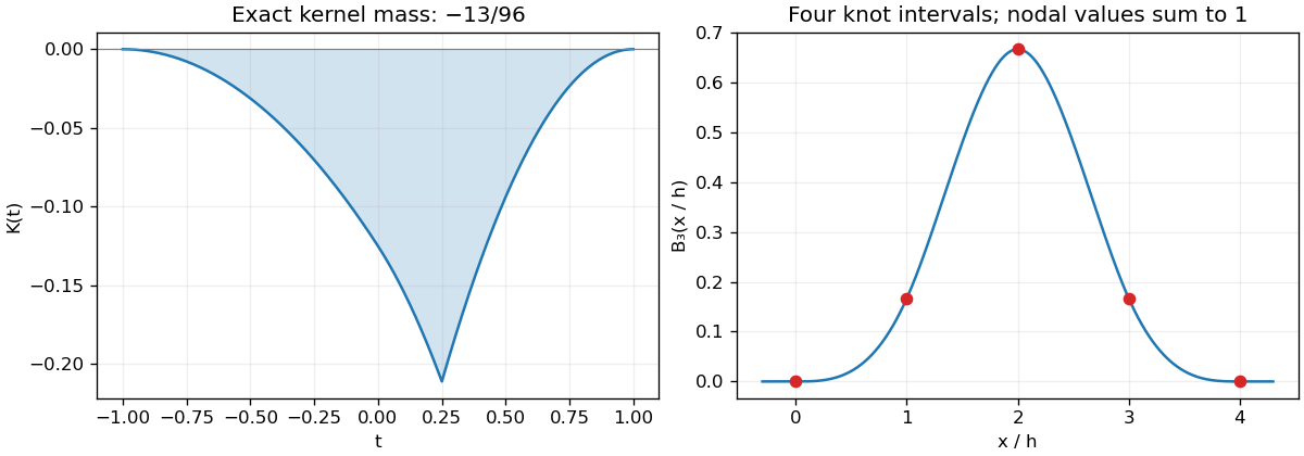
The negative Peano kernel fixes the sharp error constant, while the normalized compact cubic B-spline spans four knot intervals
. Details. 
A cubic spline that vanishes for and is twice continuously differentiable can be written using truncated power functions as . Vanishing for imposes the four moment equations for . Their Vandermonde matrix has rank , so a nonzero coefficient vector first exists at .
A normalized compact cubic cardinal B-spline isIt has nodal values at , so their sum is one. The alternating binomial coefficients meet the four moment equations, and the factor fixes the requested normalization.
For interpolation on , centre the translates as , with . Their restrictions form a basis for the cubic spline space on these knots. Write . The interpolation equations areThe recurrence determines all remaining coefficients after choosing , giving exactly two free parameters. The two natural cubic spline conditions becomebecause .
For uniqueness, take the difference of two candidates. It vanishes at every knot and has . Integrating by parts twice on each cubic piece gives : terms involving vanish at the knots, and those involving cancel at internal knots and vanish at the endpoints. Thus ; the remaining affine function vanishes at both endpoints and is zero. The square linear system for the coefficients is therefore nonsingular, giving existence as well as uniqueness of the natural cubic spline interpolant.
Let . If minimizes the squared L2 norm error, then for any the real quadratic has its minimum at . Its derivative there is zero, giving .
Conversely, if is orthogonal to , then for every , and the Pythagorean theorem for inner product spaces givesThis proves the equivalence and identifies as an orthogonal projection. It characterizes a minimizer whenever one exists; a general nonclosed vector subspace need not admit a projection for every .
The orthogonal projection is . Subtract it from and use the orthonormal basis relations to obtainThis is the requested Bessel inequality.
For the infinite tail, use completeness of the orthonormal polynomial family in the usual weighted L2 space. The relevant density facts are that continuous functions are dense for the finite measure , and the Weierstrass approximation theorem makes polynomials uniformly dense in continuous functions on the compact interval. Since , uniform approximation also gives weighted L2 norm approximation. Parseval's identity therefore givesHere finiteness of the weight integral is also necessary for the constant polynomial to belong to the stated Hilbert space. Without completeness of the polynomial family, an additional squared component orthogonal to every polynomial would remain; Bessel inequality alone does not justify equality.
The moments are . The Gram-Schmidt process first gives the constant . Removing the constant component of gives , with squared norm , hence .
For the quadratic, imposing orthogonality of to one and gives and . Thus , whose squared norm is . Taking positive leading coefficients, the first three orthonormal polynomials are
For , is orthogonal to every polynomial in , so . The Cauchy-Schwarz inequality givesUsing the tail identity from part (b) and shifting the index,For the stated power law and , the decreasing-function integral test givesConsequentlyThe assumption is sufficient; this summation estimate itself only needs .
Put and . If the best uniform approximation had error below , the values of would strictly alternate in sign at all reference points. The intermediate value theorem would give at least distinct roots of a polynomial of degree at most , a contradiction. If the lower bound is immediate.
At least one reference point attains the global error maximum of , so . Optimality of gives the upper bound, and thereforeThis is the unequal-height version of the alternating-reference error bound.
Here the exchange point lies between adjacent reference points and has the same, positive error sign as the point it replaces. Hence the new set remains spatially ordered, and the old error at its points alternates in sign. Its magnitudes are everywhere except at , where .
Set . Apply the order- divided difference to and ; both vanish because their degrees are at most . In the new alternation equations, all products have the same sign. Thus the single-point exchange in polynomial minimax approximation givesThe Remez algorithm repeatedly solves for the reference polynomial and common signed height, locates a larger error extreme, and performs an order-preserving exchange. The reference height bounds the optimum from below and the global error maximum bounds it from above. Their gap provides an optimality stopping certificate. A general implementation also needs the endpoint exchange rule when the new extreme lies outside the reference set.
For a line , the error is strictly convex. Its two endpoint maxima must agree, giving . Its unique interior minimum is at . Equating its magnitude to the endpoint error givesThe errors at are respectively . The equioscillation theorem therefore certifies this best uniform approximation directly.
For degree above one, subtracting a general polynomial does not preserve convexity of the error. The required alternating extreme points include additional unknown interior points, and their derivative and equal-height equations form a coupled nonlinear problem. The simple endpoint-and-single-minimum calculation therefore does not extend as a direct higher-degree recipe.
The first-order Sobolev space is , with derivatives understood as weak derivatives and norm squared .
The printed normal boundary condition must be distinguished from a conormal condition. Take symmetric positive definite, as required for the symmetric matrix requested later. Integration by parts givesThe natural boundary term contains the conormal derivative , not the ordinary normal derivative . On a smooth boundary, writing for its unit tangent, the literal condition leaves the term , where . Its weak form therefore retains a boundary pairing:Here the tangential derivative of the Sobolev trace can be interpreted in and paired against on a smooth boundary. This form is generally nonsymmetric; the requested usual symmetric energy construction does not follow from the literal boundary condition.
For an explicit failure of the claimed mean-zero compatibility, take the unit disk, and . It has on the circle, butThus replacing the printed normal condition by a zero conormal flux is not harmless.
For the intended zero-conormal derivative problem, the requested variational and finite element conclusions are as follows. Seek withPutting gives . On a connected domain this condition permits a solution unique modulo constants; the Poincare-Wirtinger inequality gives coercivity after fixing the mean.
The energy is . A minimizer satisfies . Conversely, a weak solution satisfiesso it is a minimizer. Testing by gives the minimum valueThis value is independent of the arbitrary additive constant when . If the compatibility fails, constant shifts make unbounded below.
Write . The Galerkin method givesSymmetry of gives . For , . Equality forces constant by positive definiteness and connectedness. Since the basis sums to one, the coefficient vector represents that constant, givingThus the stiffness matrix is symmetric positive semidefinite and singular; the displayed compatibility condition is necessary and sufficient for the finite system. Positive definiteness of controls every gradient direction, preventing additional zero-energy directions and supplying ellipticity. A degenerate coefficient can introduce further kernel modes, while an indefinite one destroys the minimizing-energy argument.
Take the affine trial space and the test space . Multiplication by and integration by parts incorporate the right Neumann boundary condition as a load:For the continuous piecewise-quadratic trial space, impose the left value exactly and use the same equation for every piecewise-quadratic test function vanishing at . With a basis of that test space and , the finite element equations areThe Endpoint Poincaré inequality, reflected about the interval midpoint, makes the derivative norm a norm on . Galerkin orthogonality then gives the exact best-approximation identity: for every admissible ,Therefore minimizes the derivative error over all admissible piecewise-quadratic functions.
To prove the requested error bound, assume . Then and . We need an elementary Poincare-Wirtinger inequality on each element of length : if has mean zero, its continuous representative has a zero somewhere, and the fundamental theorem of calculus and Cauchy-Schwarz inequality give .
Choose an affine function whose slope is the average of on and whose average equals the average of . Then and both have mean zero. Applying the just-proved bound twice yieldsDefine a quadratic interpolant on by integrating from the true left-endpoint value. The equal-average condition ensures that it reaches the true right-endpoint value, so these pieces join to an admissible continuous piecewise-quadratic function . Sum the squared estimates and use the best-approximation property:Only the maximum element length is used; equal spacing is unnecessary.
For the Aubin–Nitsche duality argument, let and solve , , . Explicitly , so . Integration by parts and Galerkin orthogonality givewhere is its nodal piecewise-linear interpolant, which belongs to the quadratic test space. On each element is the average of , so the same mean-zero inequality gives . Canceling when nonzero proves the additional order:
The bilinear square finite element contains the terms . In anticlockwise corner order beginning at , its shape functions areThe mass matrix has entries . Each product separates into one-dimensional factors, with and . Diagonal, adjacent-corner and opposite-corner entries are respectively , , . ThusNumber global grid nodes by , with , and . For an interior node, four elements contribute to its diagonal, two to each axial neighbour and one to each diagonal neighbour. Its global row therefore has the nine-point stencilIn the stated ordering the axial entries occur at columns and ; the four diagonal ones occur at . No boundary degrees of freedom have been removed.
For general valid quadrilaterals, use an isoparametric finite element. Map the unit square to an element by and define physical shape functions . Require a one-to-one nondegenerate map and compatible common edges. On a shared edge the map and the trace of each shape function are linear between the same endpoints; the neighbouring traces therefore agree. The assembled functions are continuous and lie in , giving a conforming finite element space. On a non-parallelogram the pulled-back functions are generally not bilinear polynomials in the physical coordinates themselves.
Articles by others on the same topic
There are currently no matching articles.