Oxford examination release ZIP. The held member is
Digital Social Research Statistics Core/2020 Trinity a14564w1.pdf; the sitting is 5 June 2020, A14564W1.The original output contains internal contradictions. Each solution distinguishes a conditional reading of a printed field from calculations based on the actually displayed counts. All six questions are covered; no unprinted age category or individual dataset is reconstructed.
Taken at face value, the printed two-sided p-value rejects equality of average political efficacy at the 5% level, with the non-employed group scoring higher. The effect magnitude and strength of evidence cannot be reported as one coherent result because the estimates, interval, test statistic and p-value contradict one another.
Let and be the expected political efficacy scores in the two employment groups in the target population. The null hypothesis is and the two-sided alternative hypothesis is . A Welch's t-test compares the difference of sample means with its standard error, estimating the two group variances separately:The reference Student t-distribution has approximate, generally noninteger statistical degrees of freedom; it does not require equality of the two variances. Observations should be independent, with finite group variances; normal distributions give the usual small-sample rationale, while large samples permit an approximate normal sampling distribution under suitable conditions. A large sample cannot correct a biased sampling procedure or dependence between observations.[ref]
Two-Sample t-Test for Equal Means by National Institute of Standards and Technology. §1.3.5.3, unequal-variance statistic and Welch–Satterthwaite degrees of freedom
A p-value is a probability calculated under the null hypothesis and the sampling assumptions: for this two-sided test it measures the probability of an absolute test statistic at least as large as the observed one. It is not the probability that the null hypothesis is true, the probability that chance caused the observed difference, or a measure of the effect size. If the significance level was chosen in advance, the printed falls just below it. This would reject at 5%, but not at 1%. The significance level describes the long-run probability of a type I error, rejecting a true null hypothesis; a type II error instead fails to reject a false null hypothesis. Statistical power is the rejection probability under a specified alternative hypothesis. None of these errors for this particular realised study can be read as a posterior probability from .
Both the printed sample means and the positive confidence interval point toward greater political efficacy in group 0, the non-employed group. Their magnitudes disagree. Subtracting the printed sample means gives scale units. Yet the printed 95% confidence interval has midpoint , not . A two-sided Welch interval is centred on the difference of sample means. This violates the consistency identities for a two-sided t-test; the interval and estimates cannot describe the same reported comparison. If the interval alone were trusted, it would exclude zero and indicate an increase between about and units, but that is explicitly a conditional interpretation. A 95% confidence interval refers to repeated-sample coverage of a fixed statistical parameter, not a 95% posterior probability for that realised interval.[ref]
There are additional arithmetic warnings. The printed at statistical degrees of freedom gives a two-sided p-value about , not . Thus taking the test statistic as authoritative would imply much stronger evidence, not merely a marginal 5% result. The employment counts sum to , but their percentages are and , not and . If those counts also apply to the two political efficacy sample means, their weighted arithmetic mean would be about , not the reported overall ; separate complete-case group sizes are not supplied, so that last cross-output comparison is conditional on a common sample. No uniquely corrected difference, standard error or interval follows from these contradictory fields.
The political efficacy summary describes a bounded observed scale from to , with median and middle quartiles and . The interquartile range is ; the overall sample mean being below the median does not, by itself, establish a particular distributional shape. These descriptive statistics cannot supply the missing coherent group variances or a standardized effect size. Even a corrected small p-value would establish an association under a statistical model, rather than a causal effect of employment. Age, other background covariates, selection bias and the quality of the political efficacy measurement remain relevant. A defensible report gives the conditional 5% decision and direction, identifies the contradictions, and withholds a single numerical effect-and-uncertainty claim until the output is checked.
Employment is observed for all 2053 listed cases. Social media use is observed for 1424 cases, with 629 missing. The age percentages describe the five visible rows, whose counts total 1730; they cannot be treated as a complete age distribution for the stated 2053 cases.
A frequency table describes category counts and their relative frequencies. The full-sample percentage uses every listed case as denominator; a valid percentage excludes missing data for that variable. A cumulative percentage adds the valid percentages up to an ordered category. The denominator matters as much as the number: a statement about respondents with recorded use need not describe every respondent.
Employment is a binary categorical variable: 1216 cases are employed and 837 are not, or about and . Neither employment category is missing in this output. Employment labels have no intrinsic numerical spacing; codes zero and one identify the two categories under a chosen ordering convention. Cumulative percentages for a nominal categorical variable depend on the arbitrary display order and add little to this two-category description.
Age groups are an ordinal categorical variable because their intervals have a natural ordering, although the grouped representation loses exact ages. Among the five visible age rows, ages 25–44 form the largest group, with , and ages 14–24 the smallest, with . The other visible groups account for , and on that denominator. About of the visible five-row count is below 45. These percentages should not be silently applied to the stated total : for example, the same cases are only of .
The age variable key advertises six categories, whereas only five appear. Their counts sum to , leaving a difference of against the printed total; the table nevertheless prints zero missing values. This is an internal source discrepancy, not permission to label those cases as a particular unseen age group or as recorded missing data. The oldest row is labelled 65+ here but 65–74 in Figure 2. Even the age percentage total has a small display discrepancy: the five rounded percentages sum to , while the printed valid total and last cumulative percentage say . The much larger count inconsistency remains after allowing ordinary rounding.
Social media use is also an ordinal categorical variable. Its six ordered categories express increasing frequency, not equally spaced measurements: averaging category labels or claiming a one-unit change has a constant time meaning would require an additional scoring convention. Among the observed responses, the mode is never, at , followed by daily, at . Weekly use accounts for , use more than once a day for , less-than-monthly use for , and monthly use for . The first three categories together comprise about of valid responses. Consequently the middle ordered response lies in the weekly category: cumulative frequency first passes one half there.
Combining the two daily categories gives of valid responses using social media at least daily. The same recorded responses are of all listed cases. The second percentage is the fraction recorded as daily users, not an estimate that classifies all missing responses as nonusers. Missing social media responses make up . The directly calculated valid fraction is ; summing the individually rounded full-sample percentages produces the printed , a minor rounding difference. With no account of the missing-data mechanism, the observed valid distribution should not automatically be generalized to those with missing use. Employment being fully observed does not make social media missingness ignorable. The substantive distributional summary must retain both the valid-response denominator and the missing-data qualification.
The displayed age groups have fairly similar employment proportions, with no coherent monotone age trend. The printed test reports no evidence against age–employment independence; recomputing from the five visible rows reaches the same qualitative conclusion. Their totals and several auxiliary fields nevertheless do not represent one consistent table.
Each row percentage estimates an employment proportion within that age group. For example, of the youngest displayed group are employed. The employed proportions in the next four rows are , , and . The largest displayed proportion is in the 45–54 group and the smallest in the 55–64 group, a difference of about percentage points. These are conditional percentages, not the age distribution of employed people. The sequence rises and then falls; there is no simple increasing or decreasing pattern.
The null hypothesis for a Pearson chi-squared test of independence is that the joint category probabilities factor into their age and employment marginals. Its expected frequencies are , and its test statistic adds the standardized squared count discrepancies, . For a complete contingency table with positive margins, the large-sample reference chi-squared distribution has statistical degrees of freedom. Independent observations and an appropriate sampling scheme are essential; adequate expected counts make the approximation more plausible.[ref]
Pearson's Chi-squared Test for Count Data in the R documentation. Details: independence null, asymptotic reference distribution and observed/expected counts
Reading only the printed test block, , statistical degrees of freedom and are mutually compatible. The printed likelihood-ratio test gives nearly the same p-value, about . At a prechosen 5% significance level neither rejects independence. This is a failure to find evidence, not proof of equal employment probabilities at every age. The printed Cramér's V around suggests a small sample association; the contingency coefficient around has the same broad message. The generalized phi coefficient is an unsigned chi-squared magnitude here, not evidence for a positive age trend. A small association magnitude and a large p-value answer different questions.
But only a table is actually visible. Those rows total , with employment column sums and , rather than the printed with columns and . Computing solely from the five visible rows givesIts likelihood-ratio test statistic is about , again with statistical degrees of freedom. The smallest count-based expected frequency is about , comfortably large for this ordinary approximation, but different from the printed minimum . These figures are a labelled analysis of the visible subset, not a repaired full dataset. An unprinted sixth age row might explain some intended metadata, but neither its label nor a uniquely justified reconstruction is supplied. The oldest printed label also conflicts with Figures 1 and 8.
The ordinal measures look for an ordered tendency. Goodman and Kruskal's gamma compares concordant pairs with discordant pairs among pairs untied on both variables. The printed negative gamma, Somers' D, Kendall's tau-b and Stuart's tau-c therefore suggest, at most, a very weak tendency toward lower employment at higher age categories under the specified ordering. Their precise magnitudes are not reliable here. The ordinary unordered-pair partition for ordinal data fails for the printed pair counts, even when compared with the printed cases. On the five visible rows the respective count-based values are about , for employment conditional on age, and . None gives a substantial monotone pattern; a near-zero ordinal measure would not exclude a nonmonotone relationship in general.
Goodman and Kruskal's lambda is zero in both predictive directions on the visible table: knowing age does not improve the number of correct predictions made by always choosing the most common employment category, and knowing employment does not improve modal age-category prediction. Zero modal-prediction improvement does not mean every category distribution is identical. Both the reported test block and the separately recomputed visible-table test fail to reject independence; neither justifies asserting no association, a causal age effect, or a coherent full-sample calculation from the contradictory printout.
Within the 1424 complete records displayed here, employed respondents report more frequent use on average in the ordinal sense of positive pairwise association. The overall independence test is significant, but its sample association magnitude is modest and the result is observational. Some printed ordinal summaries are internally inconsistent.
Compare row percentages because employment groups have different sizes. Never-use is reported by of the non-employed group and of the employed group. Daily use is versus ; more-than-daily use is versus . Combining the last two categories gives versus , an employed-minus-non-employed difference of about 11.26 percentage points. That threshold comparison is a descriptive summary of the six-category table, not a replacement for the original omnibus test or a newly declared prespecified endpoint. It does not assign equal spacing to the six frequency categories.
Here the row counts, column counts and grand total are additive. Under the null hypothesis of employment–use independence, a contingency table has statistical degrees of freedom. The Pearson chi-squared statistic recomputed from the cells is , agreeing with the printed value, and its p-value is about . The likelihood-ratio test statistic gives . Both reject independence at the conventional 5% and 1% significance levels under the sampling assumptions. The minimum expected frequency, about , gives no sparse-cell warning for this table. The tests compare whole category distributions; they do not by themselves identify one category as the source of the association or establish its causal direction.
Cramér's V is . The generalized phi coefficient coincides with it for this two-row table, while the contingency coefficient is about . These are modest magnitudes; a small p-value does not make the relationship large or useful for individual prediction. The employment–use association could change after conditioning on age or other covariates, and the sample excludes cases without recorded use. Relative to the employment margins in Figure 1, the omitted complete-case counts are non-employed and employed, or about and of those groups. Different missing fractions alone do not identify the missing-data mechanism, but they rule out treating complete records as automatically representative of everyone.
The count-based Goodman and Kruskal's gamma isWith the employment categories ordered non-employed then employed and use ordered from never to more than daily, this positive value means concordant pairs outnumber discordant pairs among pairs untied on both variables. It is not a 16.9% increase in a person's use and is not a causal effect. Reversing one ordering reverses its sign. Excluding ties can make gamma appreciably larger than tie-adjusted measures.
For use as response and employment as predictor, the cells give Somers' D about , Kendall's tau-b about and Stuart's tau-c about . The printed Somers value and tau-b should not be presented as verified calculations: the table prints second-variable-only ties, whereas its cells give . The other four pair classes agree with the cells; the printed five classes sum to , not . The source does not establish an alternative tie convention that repairs those ordinary identities. The direction remains a weak positive association under either description, but the exact measures require coherent pair counts.
Modal prediction provides another perspective. Without employment information, predicting the globally most frequent use category, never, makes errors. Predicting a separate modal use category in each employment group makes errors. Thus Goodman and Kruskal's lambda for use given employment is : about a 1.97% reduction in modal-classification errors. For employment given use the corresponding reduction is . These identify the targets explicitly; the source's row-dependent/column-dependent labels should not be used to reverse the target interpretation. The two small numbers show why an independence test can be significant while coarse modal prediction improves very little. The supported overall finding is a modest positive association among observed respondents, requiring conditional analysis and a missing-data qualification before broader claims.
Every displayed age stratum has a higher proportion of employed respondents reporting use at least daily, and each has positive ordinal association. The visible counts do not support the printed claim of a conventional significant omnibus result in any one stratum: several test fields are contradictory, and sparse cells further limit the chi-squared approximation. Age-specific significance labels do not establish interaction or causation.
Conditioning on age means comparing the employment groups within each displayed age category. Each within-row percentage estimates a use distribution for that age–employment combination. This helps assess a marginal association that could reflect different age compositions, but broad age categories do not remove all residual confounding. The relevant conditional-independence null hypothesis is that employment and use are independent within every age stratum. It differs both from marginal independence and from a null hypothesis that the strength of association is identical across ages.
For the 14–24 stratum, . The non-employed group reports use at least daily in of cases, versus of employed cases: an 11.13-percentage-point difference. Daily use alone is versus . This is not a uniform upward shift at every threshold: never-use is also higher among employed respondents, versus , whereas weekly use is lower, versus . The count-based Cramér's V is about and Goodman and Kruskal's gamma about . The cells give on statistical degrees of freedom, with , agreeing qualitatively with the likelihood-ratio result , . The printed Pearson and disagree with the cells and with one another: that printed statistic at statistical degrees of freedom would give about , not . Four of twelve expected frequencies are below five, with minimum about , so an exact conditional test or a Monte Carlo test is preferable for calibrated inference rather than trusting a marginal printed significance label.
For ages 25–44, . At-least-daily use is in the non-employed group and in the employed group, a difference of 11.06 percentage points. Never-use is versus , daily use versus , and more-than-daily use versus . The count-based Cramér's V is about and Goodman and Kruskal's gamma about . The visible cells give , , and , , each with statistical degrees of freedom. These differ materially from the printed Pearson , , and printed likelihood-ratio , . Even the printed Pearson statistic at its stated statistical degrees of freedom gives , not the stated p-value. The minimum expected frequency is about , so the principal difficulty here is corrupted numerical output rather than a listed sparse-cell warning. The recomputed 5% test fails to reject independence, although its p-value is not evidence that the positive descriptive contrast is exactly zero.
For ages 45–54, . At-least-daily use is versus , a difference of 9.03 percentage points. Never-use is versus , and daily use versus . The count-based Cramér's V is about and Goodman and Kruskal's gamma about . The cells give , , consistent with the likelihood-ratio , . The printed Pearson and are incompatible with the cells and with one another: using that statistic at statistical degrees of freedom gives . The smallest expected frequency is about . Thus this is another positive descriptive contrast without a count-supported significant omnibus result at 5%.
For ages 55–64, . At-least-daily use is versus , a difference of 7.89 percentage points. Never-use is versus , and daily use versus . Cramér's V is about and Goodman and Kruskal's gamma about . The printed and count-based Pearson result agrees: , statistical degrees of freedom, . The likelihood-ratio p-value is about . Two of twelve expected frequencies are below five, with minimum about ; the nominal result does not indicate rejection, but a simulation-based check would be prudent if formal calibration mattered. Neither a large p-value nor the smaller sample establishes an absence of association.
For the oldest stratum, labelled 65+ in Figure 8, . At-least-daily use is versus , a difference of 5.61 percentage points. Never-use is versus . Cramér's V is about and Goodman and Kruskal's gamma about , the largest of the five displayed strata. Yet on statistical degrees of freedom gives , while the likelihood-ratio p-value is about . There are four expected frequencies below five, with minimum about . Sampling uncertainty and a sparse distribution therefore matter greatly; the larger descriptive ordinal magnitude is not evidence for a significant age interaction. The zero observed entries do not establish zero population probabilities. An exact conditional test or a Monte Carlo test can retain the six categories without relying on a doubtful asymptotic approximation. Collapsing categories should have a substantive justification; searching for a grouping that produces significance changes the inferential problem.[ref]
Pearson's Chi-squared Test for Count Data in the R documentation. Details: asymptotic versus simulated fixed-margin tests and the role of positive margins
The following original analytical plot summarizes a common threshold rather than reproducing any source table. Its overall reference is deliberately separated: the five age strata total , not the in Figure 3, so their percentages cannot be pooled and called the reported overall result.
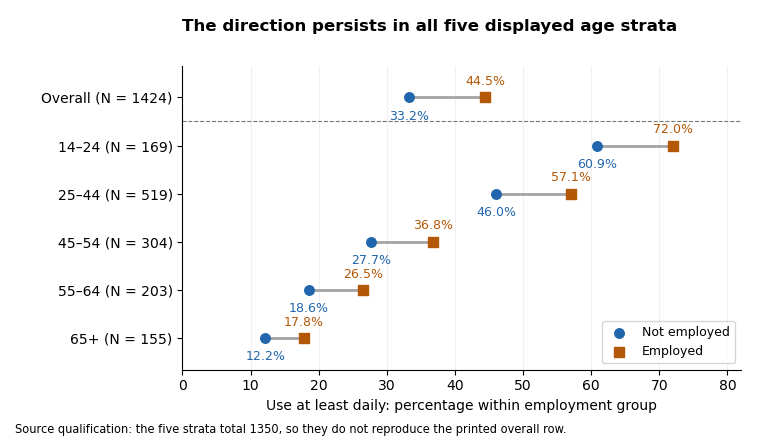
At-least-daily use is more common among employed respondents in each displayed age stratum; the printed overall row is a separate, non-reconciling input
. Details. 
Across the visible strata, frequent use declines strongly with age in both employment groups, while the at-least-daily employment difference remains positive. This is compatible with age being important to the use distribution and with a positive employment association persisting after age stratification. It is not a demonstrated Simpson's paradox: none of these displayed threshold differences reverses direction. The evidence also does not establish how much age confounds the overall result, because the strata do not reproduce its sample and the oldest age labels disagree across figures. Among young respondents the positive ordinal association coexists with a reversed never-use contrast, so the threshold summary should not be described as stochastic domination of every conditional distribution.
Ordinal measures summarize a different aspect from the omnibus tests. Counting pairs from each visible table gives Goodman and Kruskal's gamma approximately in age order. For use as response, the corresponding Somers' D values are about ; Kendall's tau-b values are ; and Stuart's tau-c values are . They are all positive and modest, but not interchangeable. Gamma discards pairs tied on either variable; Somers' D includes response ties separated by employment; Kendall's tau-b adjusts for ties in both variables; Stuart's tau-c adjusts for table dimensions. The printed second-variable tie counts violate the unordered-pair partition for ordinal data in all five strata, so the printed Somers and tau-b values should not be accepted as independently verified numbers.[ref]
Ordinal association measures in the DescTools documentation. KendallTauB and StuartTauC: distinct tie/table-size adjustments
Goodman and Kruskal's lambda for predicting the use category from employment is zero in all five visible strata: each employment row has the same modal use category as its stratum overall. This does not contradict their nonzero gamma or V, because the rest of each category distribution can change without its mode changing. Reversing the prediction target gives about for predicting employment from use. In the original display these are the second lambda values; identify the target directly rather than relying on ambiguous row/column-dependent labels. The contingency coefficient, another unsigned transformation of the Pearson statistic, adds no new direction and cannot repair a corrupted test statistic.
Even if all printed p-values were trusted, a significant result in one age group and a nonsignificant result in another would not prove that their effects differ. A statistical interaction needs a direct comparison of effects on a specified scale, not a comparison of significance labels. Five separate tests also create a multiple-testing issue if the aim is to claim at least one association; choosing categories or a threshold after inspection adds further selection. A joint conditional independence test for stratified contingency tables or an appropriate categorical-response model can target a clear combined hypothesis, with exact or simulation-based calibration where needed. Such a model would require coherent input tables before it could resolve the source discrepancies. The sound conclusion is a consistent positive descriptive tendency within the five shown strata, with no count-supported nominal 5% omnibus rejection in an individual stratum, and insufficient coherent output for a claimed causal or precisely quantified age-adjusted effect.
Read conditionally, the fitted slope says that a one-point higher skill score is associated with about 0.209 more household devices in the fitted conditional expectation. The printed summary also claims a significant slope and about 28.93% explained sample variation. Those claims cannot be assembled into one valid fitted model: several regression identities fail, so a single verified coefficient-and-uncertainty report is unavailable.
The response is a device count, while the predictor is a skill score. A simple linear regression models , where is the device count and the skill score. Ordinary least squares chooses the intercept and regression slope to minimize the residual sum of squares. The regression slope describes a conditional association, not the causal effect of training or acquiring a device.
The descriptive statistics put the device count between and , with sample mean about and sample standard deviation about among records. Skill scores range from to , with sample mean about and sample standard deviation about among records. Two missing skill values account for the stated two deleted records; because device counts have no missing values, the regression complete-case sample has observations. Estimating two regression coefficients leaves residual statistical degrees of freedom, matching that part of the output. The units of the two standard deviations differ, so comparing with does not establish that skill is more variable in a substantive sense.
If the coefficient estimates are trusted, the fitted values follow . The intercept predicts about devices at a skill score of zero; zero is within the stated score range, but precision and the number of observations near zero are not shown. A five-point increase in score corresponds to about additional fitted devices and a ten-point increase to about . At a score of ten the fitted value is about , and at 24 it is about . Expected counts may be fractional even though individual counts are integers. These are conditional interpretations of the coefficient fields, not reconstructed raw observations or validated individual predictions.
A coefficient's standard error estimates its sampling uncertainty, whereas the residual standard error describes unexplained response variation. For the intercept, , agreeing with the printed and rounded . Conditional on the model assumptions, this would reject a zero intercept at conventional significance levels. The intercept test is not a test of whether skills predict devices. For the slope, the printed would reject at 5% but not 1%; it does not assign a probability to the null hypothesis or measure the usefulness of prediction. The significance stars simply encode thresholds and add no independent evidence.[ref]
Summarizing Linear Model Fits in the R documentation. Value: coefficient, standard-error, two-sided t and p columns; sigma, residual degrees of freedom and F statistic
The slope row fails its own arithmetic check:At statistical degrees of freedom the ratio gives a two-sided p-value about , while the printed gives about ; neither is . Thus the choice of which source field is trusted changes the apparent strength of evidence, including the 1% decision. A 95% confidence interval built conditionally from the printed estimate and standard error would be about , but it is not a verified interval from a coherent fitted model. In fact, using the printed residual standard error , the complete predictor sample size and predictor standard deviation gives a slope standard error near , not .
The printed coefficient of determination would mean that the fitted line explains of the complete-case sample's centred device-count sum of squares relative to an intercept-only fit; remains unexplained by that comparison. It is not the percentage of devices caused by skill, the fraction of correctly predicted households, or a measure of future predictive accuracy. The adjusted coefficient of determination is consistent with that and the given sample size, allowing rounding. The small adjustment reflects fitting one slope among many cases; it does not validate the model.
For a one-predictor ordinary least squares fit with an intercept and the usual common-variance standard errors, the simple-regression output identities requireHere the printed slope t gives , the printed F field says , and the printed instead implies . These cannot all hold. Moreover, on and statistical degrees of freedom has p-value about , not . Reading the printed F p-value alone would give a 1% significant test of the zero-slope model, but its reported calibration is incompatible with its statistic. No significance label resolves these identities.
There is also a contradiction that does not depend on tail probabilities. Ordinary least squares with an intercept makes the arithmetic mean of fitted values equal the arithmetic mean of observed responses on the analysed records. The printed coefficients and predictor mean give . Deleting two device counts anywhere in the printed range , and allowing the reported overall mean to be rounded, would leave the complete-case device mean between approximately and . The mean bounds after deleting bounded observations therefore rule out reconciling with the response summary merely by citing those two missing predictor values. This is not the mistaken assumption that full-sample and complete-case sample means must always be identical.
If its own field were trusted, residual standard error estimates the unexplained response standard deviation, in device-count units. It is neither the standard error of the slope nor a guarantee that every prediction is accurate to devices. The residual five-number summary has extremes near and and median near , with central quartiles near and . The roughly central median does not establish normally distributed errors, homoscedasticity, independence or a linear conditional expectation. A residual-versus-fitted plot could check curvature and spread; a normal probability plot could assess an error-shape approximation. Neither diagnostic can be recovered from five residual quantiles alone. Individual prediction intervals include response variation as well as coefficient uncertainty and are wider than confidence intervals for the conditional expectation.
For conventional finite-sample t and F calibration, a normal linear model assumes independent mean-zero normal errors of common variance with an appropriate predictor specification. Mean-zero errors conditional on skill and adequate sampling remain essential even when large-sample approximations relax normality. A bounded count response can have nonconstant conditional variance, so residual diagnostics and a scientifically suitable response model matter; count data do not become normally distributed just because the sample is large. Poisson regression is one possible alternative to investigate, but its own conditional mean–variance assumptions and the bounded device range require assessment, not automatic substitution. Complete-case selection can also bias the fitted association if it depends on the response in a relevant way. The only safe summary is conditional: the printed slope is positive, but the numerical effect, its standard error, t/F evidence and explanatory fit require a corrected, coherent output before a single definitive regression claim is made.
Articles by others on the same topic
There are currently no matching articles.