Original public paper: Physical PDF pages 596–597. Both long questions and all four optional notes are covered.
Bayes' theorem relates a model parameter and observed data by . The posterior describes the parameter after observation, the likelihood describes the data for a specified parameter, the prior describes the parameter before these data, and the evidence normalizes the posterior. Likelihood is a function of the unknown parameter; it is not automatically a normalized probability density over that parameter.
Stellar parallax is the apparent annual change of a nearby star's direction relative to distant background objects as the observer moves around the Sun. The conventional parallax angle uses a one-AU baseline, so in radians, or in parsecs and arcseconds. Many small approximately independent centroiding and reference-frame errors can yield approximately Gaussian parallax errors through the central limit theorem. Correlated calibration errors, outliers and low-signal image fitting can violate that approximation; Gaussian measurement errors also need not produce Gaussian errors after taking a reciprocal distance.
For a locally uniform spatial population, the number in a spherical shell is proportional to . Changing variables using givesThis is a local population-density rule on its valid distance range. It needs a finite population or survey boundary to be a normalized global prior. An unbounded volume prior combined with a Gaussian parallax likelihood can otherwise yield an improper posterior, as explained by the proper distance prior for parallax inference.
For the requested top-hat calculation, distinguish the unknown true parallax from the reported likelihood center . Take a known fixed half-width , so the likelihood is constant over . Assume this interval lies inside the applicable population range. The top-hat parallax posterior under a uniform-volume prior is thenSetting givesThe greater available volume at smaller true parallaxes weights that side of the likelihood more strongly. This inference is not an additional measurement of the star's actual parallax.
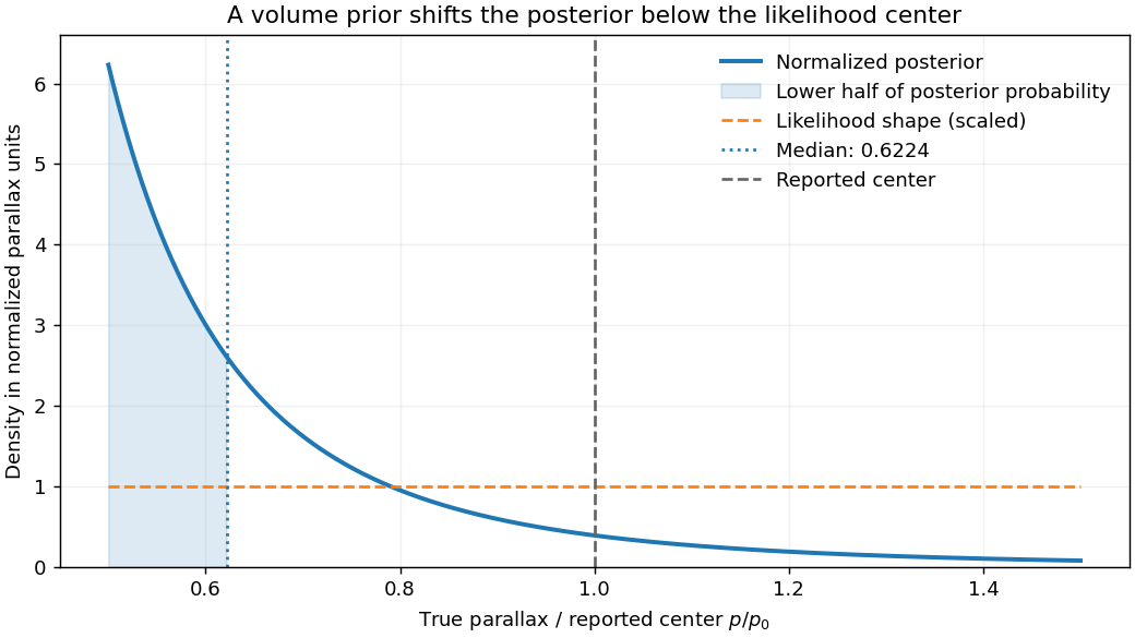

The printed notation uses both for the unknown true parallax and for the top-hat center in the numerical comparison. The distinct notation above states the consistent fixed-width interpretation yielding its result. If the half-width instead varies with the unknown parameter as , the normalized likelihood has an additional factor and different support; the same posterior calculation cannot be reused unchanged.
To improve distance inference, use independent information on luminosity, spatial density, extinction and sample selection. If the common luminosity in the measured band is calibrated, a flux measurement supplies another distance constraint through . If that common luminosity is unknown, it can be treated as a population parameter rather than silently assumed known. A finite distance distribution and the actual selection function specify which prior is appropriate. The classical Lutz-Kelker bias is a sample-calibration problem; a posterior shift under a justified prior is not itself an error to remove by a universal correction.
With flux-limited selection for identical standard candles and a noise-free threshold, there is a maximum observable distance, hence a minimum true parallax. The selected prior is truncated there. There is no luminosity-preference Malmquist bias if every object truly has the same luminosity. With a luminosity distribution, the accessible Euclidean volume scales as , preferentially including brighter objects; this is the Euclidean accessible-volume luminosity weighting underlying Malmquist bias. Flux errors additionally scatter numerous faint sources upward across a threshold, biasing selected measured fluxes. Extinction, different spectral energy distributions in a selection band, crowding, completeness and parallax-quality cuts can alter the effective population. These effects require a joint selection and error model rather than a single blanket parallax correction.
The wavelength is . Thirty dishes give interferometric baselines. The longest projected baseline sets the finest angular scale, while the individual dish beam sets the instantaneous field of view. At the maximum separation,A aperture instead has primary-beam width of order , about arcseconds; the Airy first-null convention gives about arcseconds. Illumination taper changes the precise beam definition. The array therefore resolves many synthesized beams within one pointing, but it does not image an arbitrarily wide field at that resolution.
The shortest useful baseline determines missing large-scale structure. A common estimate is . If dishes can be packed with usable center separations near , this is of order arcseconds. A more extended layout has a smaller recoverable scale. The site diameter does not specify or the actual Fourier coverage, and low-elevation shadowing can remove short spacings. Mosaicking expands sky coverage but does not supply all zero-spacing information; suitable total-power or compact-array data help recover extended emission. Earth rotation and reconfiguration improve sampled baseline coverage, sidelobes and image reconstruction, with a tradeoff between resolution and surface-brightness sensitivity.
For dish aperture efficiency , . The system-equivalent flux density of one dish isFor independent receivers, natural weighting, correlator efficiency and equally sensitive polarization products contributing to intensity, the unresolved-source thermal rms isHere is usable bandwidth and integration time. A numerical sensitivity is therefore conditional on these unspecified observing choices. For an illustrative bandwidth, one hour, two polarizations and , it is about , or at . Resolved-source brightness sensitivity also depends on beam area and missing flux. The sensitivity expression assumes naturally weighted data and the stated polarization convention.[ref]
Earth rotation changes geometric delay. At a baseline , can be of order , here , and a raw fringe-rate bound isThe actual rate depends on geometry and source direction. Correlator delay tracking and fringe stopping compensate the chosen phase center rather than averaging rapidly rotating uncorrected fringes away. Off-center directions retain residual delays and rates.
Finite bandwidth causes chromatic phase averaging and radial bandwidth smearing. A direction offset has residual delay of order ; a channel should satisfy for small decorrelation. Across a field of order radians on the longest baseline, the one-cycle frequency scale is about , so substantially narrower channels are required for accurate wide-field imaging. Similarly, time averaging should keep ; the associated one-cycle scale is about seconds in this example. Frequency-resolved visibilities and shorter dumps control these field-dependent averaging losses in radio interferometry; they are averaging losses, not ordinary glass-lens chromatic focusing.
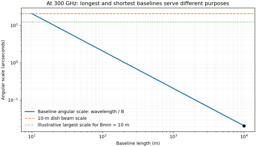
Millimeter-array baseline tradeoff: angular resolution and the loss of large-scale structure
. Details. 
At , atmospheric water vapor produces absorption, thermal emission and path-length fluctuations. A high dry site reduces these effects, while phase fluctuations can still destroy coherence on long baselines. A one-radian phase corresponds to path fluctuation , motivating frequent phase calibration or atmospheric path monitoring. Surface errors must also be small relative to the wavelength: the Ruze efficiency factor is . Pointing errors matter relative to a primary beam only tens of arcseconds wide.
Important systematic errors include antenna gains and bandpasses, delay and baseline-coordinate errors, polarization leakage, pointing, atmospheric opacity, correlator response and flux-scale calibration. Nearby compact calibrators, bandpass standards, appropriate total-power information and repeated configurations address different parts of this problem. High nominal collecting area and longest-baseline resolution alone do not determine image dynamic range or reliable extended-source flux.
Forbidden emission lines arise from transitions strongly suppressed in the electric-dipole approximation, often between metastable levels. They can radiate in dilute gas because collisions are infrequent enough for a slow radiative decay to occur. In a two-level optically thin approximation, statistical equilibrium givesThe critical density of an atomic transition is . At densities well below it, almost every collisional excitation radiates; above it, collisional de-excitation quenches the line relative to its low-density scaling. Collision coefficients and level populations determine the detailed multi-level diagnostic.
To measure temperature, compare lines of the same ion with significantly different upper-level excitation energies. The excitation coefficient contains a factor roughly times a collision strength. The oxygen forbidden-line temperature diagnostic compares the relatively high-excitation -angstrom line with the strong - and -angstrom lines. Their ratio is sensitive to electron temperature while canceling much of the common ionic abundance and emission measure.
To measure density, use upper levels with similar excitation energies but different radiative lifetimes and critical densities, as in . Their relative collisional quenching changes the ratio over an intermediate density range. At very low and very high densities the ratio approaches limiting values and loses sensitivity. A practical analysis fits density and temperature together, corrects wavelength-dependent extinction and calibration, checks blends and optical-depth assumptions, and uses reliable atomic transition and collision data. A single measured ratio generally constrains an emitting-gas model rather than proving every point of a nonuniform nebula has the same temperature.
The thermal Sunyaev-Zeldovich effect is inverse-Compton scattering of cosmic microwave background photons by hot electrons in the intracluster medium. Electron thermal energy shifts photons toward higher frequencies, changing the spectrum relative to neighboring sky. In the nonrelativistic, small-optical-depth limit its amplitude is controlled by the Compton parameterIt measures line-of-sight electron pressure. At low frequencies the apparent Rayleigh-Jeans temperature changes by . The thermal spectral distortion crosses through zero near for the usual CMB temperature and then becomes an increment; relativistic corrections matter for hot gas. Multi-frequency measurements distinguish this spectrum from dust, radio sources and an ordinary CMB temperature fluctuation.
The surface-brightness contrast has no ordinary dimming for the same cluster pressure integral: the incident CMB temperature and the observation's frequency redshift scale together. Angular extent and integrated flux still depend on distance. This makes the effect useful for selecting distant clusters and mapping their thermal pressure. The solid-angle integral scales with total thermal energy divided by angular-diameter distance squared, providing a mass proxy when its gas-physics calibration is specified.[ref]
Planck 2013 results. XXIX. Planck catalogue of Sunyaev-Zeldovich sources by Planck Collaboration. cluster survey and integrated-SZ selection context
X-ray surface brightness depends roughly on , whereas depends on . Combining X-ray spectra, brightness and resolved SZ data constrains density and line-of-sight depth. With a justified geometry, comparison to angular size gives a distance estimate; clumping and elongation can bias it. Cluster abundances and their redshift evolution test cosmological structure growth after selection and mass calibration are modeled.
The kinetic Sunyaev-Zeldovich effect additionally probes bulk line-of-sight motion, with leading in a stated velocity-sign convention. Its approximately blackbody temperature spectrum differs from the thermal distortion. These are complementary measurements of thermal pressure and gas motion, requiring foreground and instrumental control.
A charge-coupled device converts incident optical photons into collected electrons in pixel potential wells. Exposure accumulates charge; clocked transfers move it to readout amplifiers. Quantum efficiency, gain, read noise, dark current, saturation and charge-transfer behavior determine the usable signal. Bias or overscan estimates remove electronic offsets, dark frames characterize dark signal where needed, and flat fields correct relative response and illumination. Multiple exposures help identify cosmic rays and defective pixels, while astrometric alignment permits stacking.
For aperture photometry, sum the source aperture and subtract an estimated local sky contribution. A point-spread-function fit can instead use the expected spatial shape, particularly in crowded fields. Detector gain converts recorded units to electrons before applying a Poisson noise calculation. Let the aperture contain pixels, total expected source charge , sky charge per pixel, dark charge per pixel and rms read noise per pixel. With a perfectly known background mean,If the background is estimated from independent comparable blank pixels, its subtraction adds approximately , givingThe extra term is uncertainty in the estimated mean; it does not replace the sky shot noise already present in the source aperture. A more exact budget propagates the actual bias, dark and flat calibrations and any pixel correlations. The existing aperture photometry with an estimated background derives this distinction.
For one exposure in the photon-limited regime, signal grows as and its counting noise as , so SNR grows as . Read-noise domination can favor longer individual exposures, but full-well saturation, cosmic rays, tracking and changing sky constrain them. Extraction uses an aperture correction or a calibrated PSF model to recover light outside the measured region. Flat-field errors, nonlinearity, imperfect sky gradients, blending and atmospheric transparency can dominate bright-source accuracy even when the formal photon error is tiny.
Type Ia supernovae are standardizable candles. Multi-epoch photometry measures peak brightness, light-curve shape and color; spectroscopy identifies the supernova type and supplies a redshift, preferably also using the host. Correcting the empirical width–luminosity relation and attenuation reduces the spread of absolute magnitudes. A nearby sample fixes a distance-ladder intercept, while distant events test the shape of the Hubble diagram. The observable relation isAn unknown common remains degenerate with the Hubble-constant intercept unless externally calibrated; relative distance-versus-redshift shape can still constrain acceleration.
For a cosmological spacetime described by an FLRW metric, the deceleration parameter is , and the low-redshift luminosity-distance expansion isA range of redshifts therefore tests the expansion history beyond the leading linear Hubble law. Within conventional matter-plus-cosmological-constant models, standardized distant supernovae fainter than a specified decelerating prediction imply larger luminosity distances and can favor . For late-time matter and a cosmological constant, . A flat example has . One brightness residual alone does not establish acceleration across arbitrary expansion histories or arbitrary attenuation models.
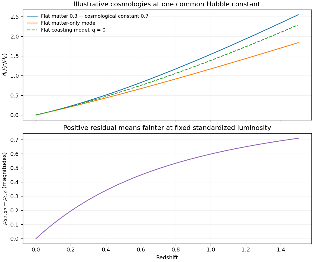
Illustrative luminosity-distance curves: expansion histories change standardized supernova magnitudes
. Details. 
The supernova discovery of accelerating expansion combined repeated imaging, difference-image candidate searches, spectroscopic classification and calibrated light curves. In the High-Z survey, CCD discovery images and later host images separated transient light from its host; point-spread-function fitting and artificial-star recovery tests checked the photometry. The measurements require K corrections between received and emitted passbands and account for the observed stretching of light-curve times.[ref]
Observational Evidence from Supernovae for an Accelerating Universe and a Cosmological Constant by Adam Riess and others. Sections 2.1–2.2, discovery imaging, spectroscopy and photometric controls
Relevant systematic tests include dust and color laws, possible population evolution, flux-limited selection, calibration across filters and telescopes, gravitational lensing and host contamination. An accelerating interpretation is assessed by fitting a specified cosmological family and its nuisance parameters, checking those effects and comparing independent observations. The two principal discovery teams provided independent distant-supernova analyses, including the 42-event Supernova Cosmology Project result.[ref]
Articles by others on the same topic
There are currently no matching articles.