Because is arc length, . Thus , where is the unit tangent to the elastic ray. In an isotropic medium this is also the wavefront normal. Consequently is the vector slowness, of magnitude ; locally , with the travel time and the wavevector.
For depth-dependent wave speed , the ray equation gives . The horizontal component of therefore has a fixed direction, and the elastic ray lies in the vertical plane determined by that direction and its initial point. A vertical elastic ray is the limiting case. If is the angle to the vertical, its conserved horizontal slowness givesAt a horizontal interface, matching the tangential wavevector at fixed frequency gives the same invariant on both sides: this is Snell's law.
For radial wave speed , take the cross product of position with slowness. The ray equations givesince the second vector is radial. A nonzero constant is perpendicular to every position on the elastic ray, so the ray lies in a fixed plane through the centre. Radial rays obey the same conclusion with a nonunique plane. The spherical elastic ray invariant is thereforewhere is measured from the radial direction. Across a spherical interface the radius is common and tangential slowness is continuous, so this form of Snell's law survives an interface discontinuity.
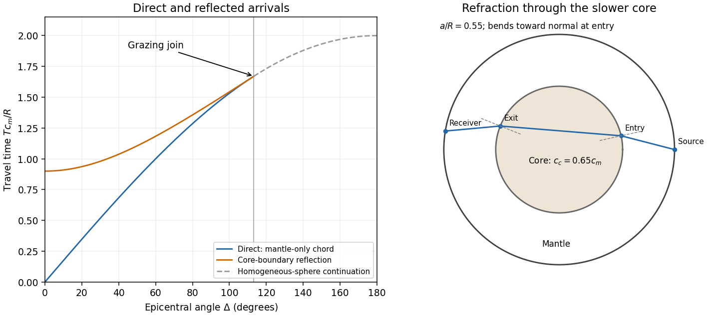
In a homogeneous sphere a P wave follows the straight chord between the two surface points. If their principal angular separation is , its length is . For constant P wave speed ,Now put and denote the mantle and core P wave speeds by . Equal incidence and reflection angles put the core-boundary reflection point on the angular bisector. Each mantle leg has length given by . Hence the core-reflected travel time isThe stated domain is essential. At the reflection point the incoming line approaches from the mantle only if . Otherwise it has already crossed the core boundary. The mantle-only direct chord also exists only for , with . In this interval,so the reflected arrival is later. Its intercept is , whereas the direct intercept is zero. At grazing incidence the branches meet at , and both have slope . A continuation of the homogeneous-sphere direct formula beyond this endpoint is not a mantle-only arrival in the modified model.
The core-transmitted elastic rays consist of three straight legs. Their impact distances in mantle and core are and , respectively. At core entry,Since , the elastic ray bends towards the normal on entry and away from it on exit. The mantle leg subtends at the centre, and the core chord subtends . Thus the total angular sweep along the transmitted path is . This sweep need not equal the principal separation if it exceeds ; the diagram uses a path with sweep below .

An elastic deformation is reversible: after removal of the deforming loads the material returns to its reference state, and its instantaneous stress is determined by its current deformation rather than a plastic or viscous history. In the infinitesimal approximation the displacement field gives the infinitesimal strain tensor . The Cauchy stress tensor is defined by traction on a plane of unit normal ; absence of body couples makes .
Let be the recoverable elastic energy per unit mass. The local mechanical power per unit volume isbecause the symmetric Cauchy stress tensor annihilates the antisymmetric part of the velocity gradient. Conservation of energy during the deformation gives . Since for arbitrary symmetric strain rates,Here the derivative is the gradient on the space of symmetric tensors, with the double-contraction inner product. This convention accounts for the two occurrences of each off-diagonal entry; treating six independent coordinates without their corresponding factors would give an erroneous factor of two in shear components.
Take a stress-free reference state of mass density . The Taylor series of the elastic energy starts quadratically:Using gives , the relation of linear elasticity. If the reference state has initial stress, the first-order expansion also retains that constant stress. Symmetry of stress and strain gives the minor symmetries , while equality of the mixed second derivatives of elastic energy gives the major symmetry . Thus the elastic stiffness tensor is a symmetric map on a six-dimensional strain space: there are independent coefficients.
For twofold elastic symmetry, choose the symmetry axis as . Rotation through is , and transforms the infinitesimal strain tensor into . Components are even and are odd. Invariance of elastic energy excludes every coupling between these parity classes. In the engineering strain ordering , with corresponding stress ordering , the symmetric stiffness matrix has the formIts symmetric even block has ten independent entries and its symmetric odd block has three. Hence a twofold axis leaves independent coefficients. No invariance under other rotation angles has been assumed.
For a homogeneous lossless elastic solid, insert the plane wave into the equations of linear elasticity. Put , , and . The resulting eigenvalue problem isThe minor and major symmetries make this acoustic tensor a real symmetric matrix. For a stable material it is positive-definite, so its three positive eigenvalues give three real positive phase velocities and therefore three slownesses . Coincident eigenvalues are possible, so there need not be three distinct speeds. For distinct eigenvalues the displacement polarization are orthogonal; in an anisotropic solid they are generally quasi-longitudinal and quasi-transverse rather than exactly longitudinal and transverse. Stability, or at least strong ellipticity in elasticity, is required for the assertion about positive real speeds.
The elastic slowness surface is the locus of the three vectors . Its equation isFor each wavefront normal there are three radial sheets, which may meet at degeneracies. To obtain the energy flux directly, multiply the elastic equation by . Forthe symmetry of stress gives . Thus the instantaneous elastic-wave energy flux is . With a real branch polarization , harmonic averaging givesNow differentiate along a regular slowness surface sheet and contract with . The terms containing cancel by symmetry and the original eigenvalue equation, leavingEvery tangent is consequently perpendicular to : the energy flux is normal to the slowness surface. At a degenerate point this statement is made on the limiting branches, rather than assuming a unique normal.
For completeness, equality of the mean kinetic and strain energies gives . Differentiating the acoustic tensor equation in the wavevector variables similarly givesThus the group velocity is the elastic energy velocity. The homogeneous elastic dispersion relation is degree one in , so differentiating at gives .
The elastic wave surface is the unit-time locus of these group velocities. From an impulsive point source, the propagating wavefronts at time are its sheets scaled to . A particular source may fail to excite a mode in some directions, and its amplitudes require the source polarization and geometrical spreading; the wave surface determines the arrival geometry. It does not specify all near-field motion between the radiative fronts. Geometrically it is the envelope of the planes : tangent variation gives , so is the appropriately normalized normal to the slowness surface.
In a symmetry-plane cross-section write , and . The two envelope conditions giveThe numerator is the signed curvature numerator of the slowness surface cross-section. At a simple inflection point, and . Then and are linearly independent. These are precisely the local conditions for an ordinary cusp. The slowness curvature and wave-surface cusps relation explains why a smooth nonconvex slowness surface can generate a cusped wavefront and multiple ray arrivals.
The example below uses a positive orthotropic stiffness in normalized units: , , , , and all normal off-diagonal stiffnesses zero. In the symmetry plane , its two in-plane acoustic tensor eigenvalues are , and its out-of-plane shear speed is . The in-plane shear sheet is nonconvex and produces the marked cusps; the construction uses an actual stable elastic tensor.
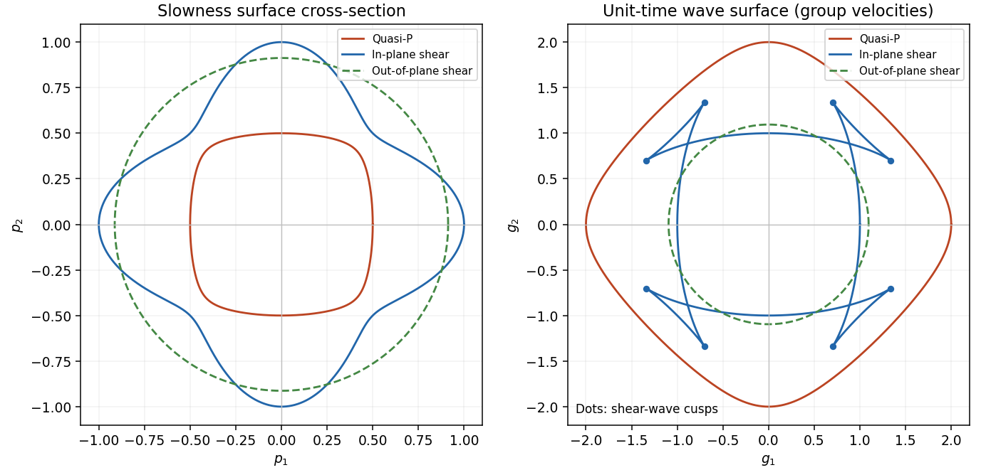
Slowness and group-velocity wave surfaces of a stable anisotropic elastic tensor, with shear-wave cusps
. Details. 
Let be the solid exterior to the cavity, and choose outward from the solid, hence into the cavity on its boundary . Subtraction of the incident solution from the total solution gives the scattered displacement field equationsThe traction-free cavity condition for the total field gives on . The scattered field has zero initial displacement and initial velocity before the pulse reaches the cavity and satisfies an outgoing radiation condition, excluding an additional incoming elastic wave. Equivalently one seeks the causal response to this prescribed boundary traction. Although the incident plane pulse extends across an infinite plane, the causal scattered field from the bounded cavity has finite propagation distance at each finite time.
To prove energy uniqueness for traction-driven elasticity, take the difference of two solutions with the same initial conditions, body force, boundary traction and outgoing condition. It satisfiesFor a large enclosing ball , multiply by and integrate over . Integration by parts givesSymmetry of stress replaces the last derivative by , and major symmetry of the elastic stiffness tensor makes that integral the derivative of the strain energy. ThereforeThe cavity contribution is zero. On any fixed finite time interval choose beyond the causal support of the scattered difference; the outer contribution is then zero as well. This gives conservation of its nonnegative elastic energy. Positive mass density and positive strain energy imply that zero initial energy forces everywhere; the zero initial displacement field then gives . The same argument works for finite-energy outgoing solutions by taking the limit of enclosing surfaces and excluding incoming energy. Hence the causal scattered field is unique. Specifying the incident field and cavity traction alone without the initial and outgoing conditions would not establish uniqueness.
Use fixed spatial coordinates in a stationary heterogeneous Earth and define the operatorHere the elastic stiffness tensor has its minor and major symmetries, and the physical body force per unit volume is . The retarded elastodynamic Green tensor is the displacement in direction due to a unit physical force impulse in direction at :It satisfies the actual Earth's homogeneous boundary conditions, including zero traction on the free surface and continuity of displacement and traction at bonded internal interfaces. Integration through gives , with . No spherical symmetry is required.
For zero initial conditions, form the convolutionApplying to this expression uses the defining Dirac delta function to give . Causality gives zero initial conditions, and each Green column supplies the required boundary conditions. The positive-energy uniqueness argument then identifies this expression with the physical response. The source factor is because is force per unit mass, whereas the Green tensor was normalized to unit force.
A force dipole is a limiting pair of opposite point forces separated by a small vector. Put at and at , and hold fixed as . Expansion of the two Dirac delta functions givesIts resultant force is zero, and integration by parts gives its radiated displacement as . Thus the source derivative of the elastodynamic Green tensor represents a dipole with force direction and separation direction .
For the surface source choose a normal from the minus side to the plus side and defineThe same normal is used in both tractions. If the elastic coefficients are continuous through the surface, the distributional gradient of a piecewise smooth displacement is . Its stress therefore has a singular part . Taking the divergence includes the regular stress jump, so a field satisfying the source-free equations on both sides has equivalent sourceIn particular, the signs follow from the chosen jump convention, not from an unspecified orientation. The elastodynamic surface-jump representation is consequentlywith the Green tensor evaluated at . The first term is a surface distribution of forces, and the second is a surface distribution of dipoles.
One can derive the same formula without multiplying discontinuous material coefficients by a surface delta. Apply integration by parts on the two sides of to the field and the reciprocal Green field . Major symmetry cancels the volume strain terms; the spatial identity iswhen the temporal terms are handled by the retarded time convolution. More explicitly, take , extend the zero-initial-data solution causally to , and integrate over all source times. Integration by parts cancels the two temporal terms, with zero endpoint terms; the causal supports subsequently reduce the representation to . The Green impulse contributes on the left. The two outward face normals are and , so their sum on the right is . Moving it to the other side gives . The same identity applied to two force Green fields with interchanged source and receiver proves the reciprocal relation ; hence the displayed surface formula follows. On a bonded material interface the Green displacement and common Green traction are continuous: is then the unambiguous version of the dipole term, evaluated with the matching one-sided coefficients. External free-surface terms vanish because both tractions vanish.
For a fault in isotropic material, the Lamé parameters giveTangential slip obeys , and ordinary fault traction is continuous across the two faces. Therefore the source is a double-couple fault source withFor a uniform patch of area with and , its integrated seismic moment tensor isThe dipole is a force in the slip direction separated in the normal direction; the dipole is a normal force separated in the slip direction. Their equal and opposite torques cancel. The symmetric trace-free seismic moment tensor has eigenvalues , with zero resultant force and torque. A temporal stress drop on a fault is not a jump of traction between its two simultaneously matching faces; it does not add a single-force layer to this tangential-slip representation.
Articles by others on the same topic
There are currently no matching articles.