Past exam of the mathematics course of the University of Cambridge / 2004 / iii / Paper 33 (Mathematics of Operational Research)

For the linear program in maximization form, a nonnegative multiplier $y$ of the resource inequalities giveswhenever $A^{T}y\ge c$. Equivalently, the Lagrangian is $b^{T}y+(c-A^{T}y{)}^{T}x$; its supremum over $x\ge 0$ is finite exactly when $A^{T}y\ge c$. Minimizing this bound gives the dual linear programThe displayed inequality proves weak duality directly.

For the final simplex tableau, the basic-variable order is $(x_2,x_1)$. With $z_1,z_2$ interpreted as the ordinary unpriced slack variables, its constraint equations giveThe bottom row is read in the reduced-cost convention $r_j=c_j-c_B^T{B}^{-1}{A}_j$, with right side minus the basic objective value. It says the reduced costs of $z_1,z_2$ are $0,-1/2$. Thus optimality requires $z_2=0$, while $z_1$ can increase without changing the objective until $x_2$ reaches zero. The complete primal optimum set is

Reconstructing a linear program from a final simplex tableau exposes a source inconsistency. The slack columns areBecause the first basic column is that of $x_2$, the original constraint data areThe slack reduced costs give $y^T=(0,1/2)$ andConsequently the recovered homogeneous linear program isEvery point in the optimum segment has value $15/2$. Since the segment contains a point with both variables positive, complementary slackness forces both dual column inequalities to be equalities. They give the unique dual optimum

The printed bottom-right entry is $-3$, but it must be $-15/2$ for this linear objective and these constraint rows. Thus no original problem in the stated homogeneous standard form has exactly the entire printed tableau. Changing that one entry to $-15/2$ gives the reconstructed problem above. Alternatively, if an affine objective is permitted, $5x_1-\frac{5}{2}{x}_2-\frac{9}{2}$ has the displayed optimum value $3$ and unchanged reduced costs; the corresponding affine dual objective is $b^{T}y-\frac{9}{2}$. Both interpretations have exactly the same primal and dual optimizer sets. The discrepancy is in the objective constant, not in the optimal segment.

True. Suppose a dual feasible solution $y$ exists. For every primal feasible $x$, weak duality gives $c^{T}x\le b^{T}y$, a finite upper bound independent of $x$. This contradicts primal unboundedness. Therefore an unbounded primal has an infeasible dual. Here “unbounded” arithmetic means a nonempty feasible set with objective values unbounded above, rather than merely an unbounded feasible region.

False: both primal and dual can be infeasible. For example, takeThe primal requires $0\le -1$, so is infeasible. Its dual requires the first coordinate of $A^{T}y$ to be at least $1$, namely $0\ge 1$, and is also infeasible. An infeasible primal therefore does not force an unbounded dual. If the dual is additionally assumed feasible, strong duality rules out a finite dual optimum; a feasible linear program with finite optimal value attains it, so in that qualified case the dual is unbounded below.

Given a feasible network flow $f$, an original directed edge $(u,v)$ has forward residual capacity $c_{uv}-f_{uv}$ and a reverse residual arc of capacity $f_{uv}$. A source–sink graph path in this residual network permits an augmentation by the minimum residual capacity along it: increase forward flows and decrease the corresponding reversed flows. Capacities and flow conservation are preserved, and the flow value increases by that amount.

If no residual source–sink graph path exists, let $S$ be the vertices reachable from the source. The sink is outside $S$. Every original arc from $S$ to its complement is saturated, and every original arc back into $S$ has zero flow, since a positive reverse residual arc would make its tail reachable. Conservation therefore givesThe flow equals this cut capacity, so the max-flow min-cut theorem proves it is maximum.

Termination needs a capacity or path-selection assumption. For integer capacities, starting from zero, every residual capacity and augmentation is integral; each augmentation increases the value by at least one, and the value is bounded by the total source-outgoing capacity. The algorithm therefore terminates. Rational capacities can be scaled to integers. With arbitrary real capacities, unrestricted graph path choices do not guarantee finite termination. A valid uniformly terminating implementation is the Edmonds–Karp algorithm, choosing a shortest residual graph path each time.

Here is why that choice works independently of numerical capacity sizes. Residual distances from the source cannot decrease after augmenting along a shortest graph path. Every newly created residual arc is the reverse of a graph path arc; if it could cause the first distance decrease, its previous distance relation would contradict that decrease. When an arc $(u,v)$ is saturated on a shortest graph path, $d(v)=d(u)+1$. Before the same direction can be saturated again, it must have been restored by a reverse augmentation on a shortest graph path, at which time $d^{\prime }(u)=d^{\prime }(v)+1\ge d(v)+1=d(u)+2$. Each arc is consequently critical only $O(|N|)$ times. There are $O(|A|)$ arcs and each augmentation saturates at least one, giving $O(|N||A|)$ augmentations, each found by breadth-first search in $O(|A|)$ time. Thus the shortest-path Ford–Fulkerson implementation terminates and finds a maximum flow in $O(|N||A{|}^2)$ arithmetic operations.

For sports elimination by maximum flow, first give the target team all its remaining wins. This cannot hurt its chance to finish strictly ahead: changing a result to favour it also removes a rival's win. Let $w^{\ast }$ be its resulting win count. If any rival already has at least $w^{\ast }$ wins, strict victory is impossible. Otherwise give each unordered pair of rivals $i<j<n$ one game node. Its incoming capacity is $g_{ij}$, and its two outgoing arcs go to the participating team nodes. Their capacities may be replaced by the finite numbersince no arc can need more than the total number of remaining rival games. Team $i$ has sink capacity $w^{\ast }-w_i-1$.

An integral flow of value $G$ saturates all game-node incoming arcs. Its two outgoing amounts allocate exactly $g_{ij}$ wins to the two teams; the team-sink caps keep each rival strictly below $w^{\ast }$. Conversely any successful completion of the league specifies such a flow. Integral capacities and augmentation give an integral maximum flow, soafter the initial negative-capacity rejection. Each actual game is counted once: making independent nodes for both ordered pairs would double-count it.

The network has $O(n^2)$ nodes and arcs. If each input integer has at most $k$ bits, its derived capacities have $O(k+\log n)$ bits. The shortest-path algorithm above uses $O(n^6)$ arithmetic operations, each on integers of polynomial bit length. Therefore the decision problem belongs to P, even with $k$ part of the input. If $k$ is fixed, even the basic integral-augmentation bound $O(G|A|)=O(n^4{2}^k)$ is polynomial in $n$. If $k$ varies, that particular bound is only pseudopolynomial; it is the shortest-path implementation that establishes polynomial bit complexity.

For a connected undirected weighted graph, a spanning tree connects all vertices without a graph cycle. A minimum spanning tree minimizes the sum of its edge weights. Disconnected input has no spanning tree, although the same methods produce a minimum spanning forest. Negative edge weights and ties cause no difficulty; a tree always contains exactly $|V|-1$ edges.

The central exchange argument is the minimum spanning tree cut property. Suppose a forest $F$ is contained in some minimum spanning tree $T$, and consider a cut with no edge of $F$ crossing it. Let $e$ be a lightest crossing edge. If $e\notin T$, adding it creates a graph cycle; the graph path in $T$ between its endpoints contains a crossing edge $f$. That $f$ is not in $F$, and $w(e)\le w(f)$. Thus $T-f+e$ is another spanning tree with no larger weight and still contains $F$. It is also minimum and contains $F\cup \{e\}$. This proves that the chosen edge is safe, rather than merely asserting a greedy choice.

Kruskal's algorithm sorts all edges by increasing weight, starts with the empty forest, and adds an edge precisely when its endpoints are in different components. Each added edge is lightest across a component cut respected by the current forest. The exchange proof inductively keeps the forest inside a minimum spanning tree; connectedness makes the final forest a spanning tree, hence an optimum. Sorting takes $O(|E|\log |E|)$ comparisons, and even a simple component-merging implementation takes only polynomial additional work. Efficient component tracking improves that overhead further.

Prim's algorithm instead grows a single tree, repeatedly adding a lightest edge from its vertex set to the outside. The same cut argument proves correctness. A dense implementation using an array runs in $O(|V{|}^2)$ comparisons. The dual minimum spanning tree cycle property says a uniquely heaviest edge of a graph cycle belongs to no minimum spanning tree: exchanging it for a lighter crossing edge strictly improves any tree containing it. Ties must be handled carefully; a merely nonunique heaviest edge can occur in an optimum.

Complexity classes are formally classes of decision problems, so use the version asking whether a graph has a spanning tree of total weight at most a supplied threshold $K$. Assume integer or rational weights and threshold are encoded in binary. The input length includes all these bits, not only the numbers of vertices and edges. P consists of decision problems decidable by a deterministic algorithm in time polynomial in that input length. NP consists of those with polynomial-size complexity certificates verified in deterministic polynomial time, equivalently decidable in polynomial time by a nondeterministic machine.

Kruskal's algorithm constructs the optimum and compares its weight with $K$. Binary integer comparisons and sums are polynomial-time operations. Rational comparisons can be made by cross multiplication, and their summed numerator and denominator have polynomially bounded bit length: a product of input denominators has bit length no greater than the sum of their bit lengths. The combinatorial algorithm makes polynomially many such operations. Hence the minimum-spanning-tree decision problem is in P; the optimization version likewise has a polynomial-time algorithm.

For membership in NP, the complexity certificate is a list of $|V|-1$ selected edges. Check that every edge is present, that the edges connect all vertices and contain no graph cycle, and that their total weight is at most $K$. A graph search and binary arithmetic do this in polynomial time. A successful complexity certificate need not establish that its tree is minimum: it proves the threshold question's yes-answer. Conversely, a yes-instance has such a tree as a complexity certificate. ThereforeMembership in NP does not arithmetic mean NP-hardness; here the explicit greedy algorithm provides the stronger tractability result.

For a transferable utility game, the characteristic function of a coalitional game assigns a coalition $S$ its largest total attainable revenue $v(S)$, with $v(\varnothing )=0$. The core of a cooperative game consists of payoff vectors $x$ satisfying efficiency, $x(N)=v(N)$, and coalition stability, $x(S)\ge v(S)$ for every $S$. A coalition receiving less could operate alone and distribute its extra value to make each member better off.

Use thousands of pounds as the monetary unit. The physical directed arcs are $A\to B$ and $C\to D$, owned by $i$, with capacities $3,2$; $A\to C$ and $B\to D$, owned by $j$, with capacities $1,1$; and $B\to C$, owned by $k$, with capacity $2$.

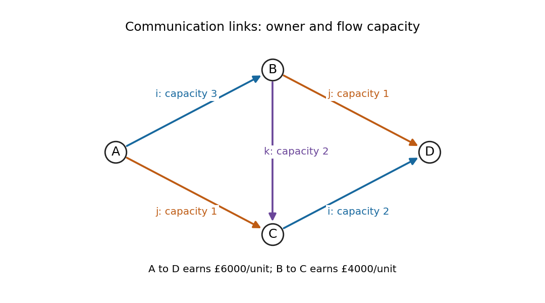
The physical network is acyclic. There are exactly three $A$–$D$ graph paths and one $B$–$C$ graph path. Let $u,v,w$ be the $A$–$D$ flows on $ABD$, $ACD$, $ABCD$, respectively, and let $z$ be the direct $B$–$C$ demand. Their capacities and revenue areEvery feasible traffic pattern decomposes into these graph paths, so these inequalities are exact. The first is redundant, since $u\le 1$ and $w\le 2$ imply it.

Formulate this as a minimum-cost flow through the two-resource path packing as minimum-cost circulation reduction. Use auxiliary vertices $s,L,R,t$ and the following arcs, whose entries are (capacity, cost):The first forward graph path carries $u$, $sLt$ carries $v$, $sLRt$ carries $w$, and $sRt$ carries $z$. Conservation at $L$ imposes $v+w\le 2$, and at $R$ imposes $w+z\le 2$; the individual finite-capacity arcs give the other bounds. The return arc closes the circulation. Its cost is exactly $-R$, so this is an ordinary minimum-cost circulation with precisely the required feasible traffic set. Unlimited capacities may all be replaced by $5$, the maximum possible total graph path flow.

An linear programming optimality certificate is particularly short:The feasible choice $u=v=w=z=1$ attains equality. Thus the actual traffic is three units from $A$ to $D$ and one from $B$ to $C$, andAll four positive terms in the bound must be tight at any optimum, so these graph path amounts are unique.

The two traffic demands must retain their identities. Merely adding fictitious return arcs $D\to A$ and $C\to B$ to the physical graph can create an invalid graph cycle combining both rewards: $A\to C\to B\to D\to A$ would credit the $j$-only network with revenue even though it carries neither requested demand. The resource-flow formulation above avoids that problem.

For the characteristic function, only complete physical graph paths owned by a coalition are available. Company $i$ or $j$ alone has no requested graph path; company $k$ carries two units of $B$–$C$ traffic. The pair $\{i,j\}$ carries one unit on each of $ABD,ACD$; the pair $\{i,k\}$ sends two units on $ABCD$ rather than selling them at the lower $B$–$C$ rate; and $\{j,k\}$ has only the two direct $B$–$C$ units. ThereforeWriting payments in thousands, all stable divisions of the revenue are exactlyEquivalently, $8\le x_k\le 10$, $0\le x_j\le 10$ and $x_i=22-x_j-x_k$. This is the entire core, not just one acceptable allocation.

The nucleolus minimizes in lexicographic order the sorted decreasing excesses of a coalition $e(S,x)=v(S)-x(S)$ over imputations. Empty and grand-coalition coalition excesses are fixed zeros and can be omitted. For the six other coalitions, efficiency givesThe two $k$-related coalition excesses sum to $-2$, so their maximum is at least $-1$. This bound is attainable, and attaining it forces $x_k=9$. All six coalition excesses are then at most $-1$ precisely when $1\le x_j\le 9$ and $x_i=13-x_j$. The fixed pair of coalition excesses equals $-1$ throughout these first-stage minimizers.

Minimize the largest of the remaining coalition excesses. They become $x_j-13,-x_j,x_j-10,-1-x_j$, whose maximum is $\max (-x_j,x_j-10)$. Its unique minimum is $-5$ at $x_j=5$. Hence $x_i=8$ and $x_k=9$. The sorted proper coalition excesses there are $(-1,-1,-5,-5,-6,-8)$, and

The total processing time ${\sum }_{i=1}^{40}{t}_i$ is constant for a single machine, so only the initial setup and changeover sum depends on the order. Use the dummy-job reduction for sequence-dependent setup times. Add vertex $0$, and setLet the binary variable $x_{ij}$ indicate that $j$ follows $i$ in the augmented tour. A Hamiltonian cycle through $0$ specifies exactly one schedule, read starting after $0$. An exact integer programming formulation isThe degree equations alone describe a cycle cover of a directed graph, possibly several separate graph cycles. The subtour elimination constraints exclude every proper directed graph cycle; the cover is therefore a single tour through all jobs. Conversely every schedule supplies a feasible tour with exactly its completion time as objective. Exponentially many written inequalities are permitted in this exact formulation; an implementation may add them only when violated.

For three parallel machines, the relevant objective is the parallel-machine makespan with sequence-dependent setups, not simply total setup cost. Partition jobs into three ordered lists ${\pi }_r$. For a nonempty list definean empty machine has $C_r=0$. Minimize $C_{\max }$ subject to $C_r\le C_{\max }$ for each machine and each job assigned once. This can be written as a mixed-integer extension with assignment variables, one dummy tour per machine and conditional subtour cuts.

A practical strategy starts with a balanced assignment, sequences each machine using the single-machine methods, and improves by relocating or swapping jobs between machines together with within-machine 2-opt moves. Score each move by its change in ${\max }_r{C}_r$. Branch and bound can combine machine-assignment decisions with within-machine assignment bounds. For nonnegative times, the total processing time divided by three and the largest individual processing time are valid lower bounds, supplemented by setup-dependent route bounds. Balancing processing and changeovers jointly is essential; independently minimizing the three tour costs does not by itself minimize completion time.

Drop the subtour elimination constraints, retaining the one-incoming/one-outgoing equations and any branch decisions. This is an assignment problem, solvable in polynomial time. Its optimum is a lower bound on the best schedule in that branch because every admissible schedule satisfies the relaxed constraints. Add the constant processing-time sum to compare completion-time bounds.

Keep a feasible schedule as an incumbent upper bound. At each branch and bound node, solve the restricted assignment problem. If it is infeasible or its bound is at least the incumbent, discard the node. If its optimum is a single tour, it is a feasible schedule attaining the bound, so update the incumbent and close the node. If it has a proper subtour $C$ with arcs $e_1,\dots ,e_r$, every valid Hamiltonian tour must omit at least one of those arcs.

For a disjoint exhaustive branching rule, child $h$ forces $e_1,\dots ,e_{h-1}$ and forbids $e_h$, for $h=1,\dots ,r$. Every valid tour falls into the child indexed by the first omitted arc. Re-solve the corresponding assignment relaxations, prioritize small bounds, and repeat. Finitely many binary choices give an exact terminating search; its worst-case tree can be exponential. Assignment optima provide lower bounds, while complete tours provide upper bounds. Patching subtours or local improvement can improve the incumbent without changing the exact pruning argument.

Represent a schedule by a permutation $v_1,\dots ,v_{40}$, with $v_0=v_{41}=0$. Choose $1\le p<q\le 40$ and reverse the block $v_p,\dots ,v_q$. This is a 2-opt move on the dummy tour. Its exact setup-cost change is the asymmetric 2-opt reversal costThe internal sum matters because the specified changeovers need not be symmetric. When the block begins at the first job, the boundary terms correctly update the initial setup; the dummy return costs are zero. Processing times cancel.

At temperature $T>0$, simulated annealing accepts a move with probabilityWith uniformly sampled reversal pairs the proposal is symmetric, so this is the appropriate Metropolis–Hastings acceptance probability. Improvements and ties are always accepted; occasional uphill moves escape local minima. Repeatedly sample moves, gradually lower $T$, and retain the best schedule seen even if the current schedule worsens. Reversing a block of length two swaps adjacent jobs, so these moves connect the whole permutation space. A cooling schedule, iteration budget and restarts control practical performance. This is a heuristic at a finite budget; it does not certify global optimality unless paired with an exact bound or an appropriate limiting convergence argument.

For pure strategy sets $S_1,\dots ,S_n$ and utility functions $u_i$, a Nash equilibrium is a strategy profile $a$ such thatFor mixed strategies, replace payoffs by their expectations under independent randomization and allow each player to choose any probability distribution. Since expected utility is linear in a player's own distribution, checking all pure deviations suffices.

Pure equilibria need not exist. In matching pennies, player 1 receives $1$ for equal choices and $-1$ for different choices, while player 2 receives the negative. At an equal pair, player 2 improves by switching; at a different pair, player 1 improves by switching. Thus no pure profile is a Nash equilibrium.

In the ranked university application game, every student must be admitted at a pure equilibrium. If someone were rejected, fewer than the total 50000 seats would be filled, so another university would have a vacancy. Moving there gives positive benefit instead of zero. Consequently all 50 universities have exactly 1000 applicants and admit all of them.

Choose a university with largest arithmetic mean admitted rank and let $r_{\min }$ be its lowest rank. If an outside student of rank $r>r_{\min }$ moved there, that student would be admitted in place of $r_{\min }$; the new arithmetic mean would exceed the university's previous arithmetic mean, which was at least the student's current payoff. This is a profitable deviation. Therefore no higher rank is outside: that university consists of the highest 1000 ranks. Remove that block and repeat with the remaining university of largest arithmetic mean. At each step the same argument excludes omitted higher ranks from the remaining set. The admitted cohorts are necessarily the consecutive blocks

Conversely, assigning these blocks to labelled universities is an equilibrium. A student moving to a higher block is rejected. A student moving to a lower block displaces its lowest rank; all the other admitted ranks there are below every rank in the student's original block. Comparing the two arithmetic means with that student's own rank held fixed shows a strict loss. Thus every block assignment is an equilibrium, and the preceding argument excludes all other pure ones:

There is more than one further mixed equilibrium. We give two genuinely mixed profiles, rather than count the pure equilibria as degenerate mixed ones. First, let every student apply independently and uniformly to all 50 universities. For each fixed student the other players' distribution is invariant under every permutation of university labels. All 50 pure applications therefore give the same expected utility. Uniform mixing is a best response, so this is a Nash equilibrium.

For a distinct mixed equilibrium, assign each of the 48 highest consecutive rank blocks deterministically to a different university. Let each of the lowest 2000 students independently choose either of the two remaining universities with probability $1/2$. For a low-ranked student these two universities have identical expected utility by label symmetry, and that payoff is positive: there is a positive-probability event on which the student is admitted. Applying to one of the 48 full higher-ranked blocks would guarantee rejection. Hence the specified mixture is a best response.

For a student in a deterministic higher block, moving to another deterministic block loses by the pure-equilibrium comparison above. It remains to rule out a move to a mixed university. Let the student's own block start at $L\ge 2001$, and let their rank be $r\le L+999$. Their present payoff is $L+499.5$. The number $M$ of low-ranked applicants at a specified mixed university has a binomial distribution with parameters $(2000,1/2)$, and the higher-ranked deviator is always admitted. If $M\ge 1$, all other admitted ranks are at most 2000, so the new arithmetic mean is at most $(r+2000)/2$, and thus at most $(L+2999)/2$. If $M=0$, it is $r\le 50000$. Therefore the expected deviation payoff is at mostbecause the gap without the last term is $(L-2000)/2\ge 1/2$. No such deviation improves the payoff. This proves a second mixed equilibrium, with only the lowest 2000 students randomizing. It is visibly different from the fully uniform profile. In particular,