A linear connection on a manifold is a rule for differentiating vector fields which is additive, is -linear in , is real-linear in , and obeys . It extends to covector fields and arbitrary tensor fields by the Leibniz rule and compatibility with contraction. In coordinates,This is the covariant derivative; the affine connection terms correct the changes of the coordinate basis. A symmetric affine connection has zero torsion tensor, , or in a coordinate basis. Symmetry does not imply metric compatibility; no metric is required for this question.
Additivity of each covariant derivative immediately gives additivity of . Expanding the second derivative of a tensor product givesSubtract the expression with exchanged. The two mixed terms cancel, proving that the curvature commutator is a tensor derivation:For a scalar, . Commuting partial derivatives and using the symmetric affine connection gives . Consequently : the commutator is linear over smooth functions, not merely over constant scalars. Write in a local basis. The tensor-product rule gives , showing that its value at a point depends only on at that point. Thus it defines the Riemann curvature tensor byThe antisymmetrized second covariant derivative is itself tensorial in the derivative indices, so this pointwise map transforms as a tensor. The formula or the defining commutator gives , hence with normalized antisymmetrization.
Apply the commutator to the scalar contraction . Its action vanishes, soSince is arbitrary, . Repeated use of the tensor-product rule gives one plus curvature action for an upper index and one minus action for each lower index. In particular,The type notation in the PDF means one contravariant and two covariant indices, not a fractional tensor order.
For the first Bianchi identity, put and . The symmetric Hessian of a scalar field satisfies . Therefore the six third-derivative terms cancel inSubstituting the covector curvature action gives . At a chosen point the gradient of a smooth scalar can be any covector, soThe second form follows from the already proved first-pair antisymmetry.
For the second Bianchi identity, the same third-derivative cancellation can be organized as an operator identity. On vector-valued components set , with . Although a full second covariant derivative includes a term for its lower derivative index, that term cancels on antisymmetrization because the affine connection is symmetric. Thus , where acts by multiplication. Expanding the three nested operator commutators makes all six triple products cancel:Equivalently, the cyclic sum of vanishes. These are the covariant derivative terms on the upper and last lower curvature indices. The two remaining lower indices add . In the cyclic sum these additions cancel in pairs, using and . Hence the Bianchi identities from covariant derivative commutators giveBoth identities here apply to any torsion-free linear affine connection; the second derivation does not require choosing a metric affine connection.
The strong equivalence principle extends universality of free fall to bodies with appreciable gravitational binding energy and requires results of sufficiently local experiments, including gravitational experiments, in freely falling laboratories to be independent of their location and velocity. The Einstein equivalence principle makes the corresponding statement for nongravitational experiments; the weak principle concerns test-body free fall without significant self-gravity. In a locally inertial frame the nongravitational laws take their special-relativistic form, while internal gravitational experiments retain the same local gravitational laws and coupling constants. They are not declared to have no gravity.
In a metric description, one may set and at a point by Riemann normal coordinates, so the Levi-Civita connection vanishes there. This removes a locally uniform external gravitational acceleration, not the Riemann curvature tensor. Tidal effects between separated bodies, or accumulated over a finite-duration experiment, remain. The local limit must control both the laboratory's size and duration. Gravitationally self-bound bodies are included in the strong version, so it is stronger than equality of inertial and passive gravitational mass for ordinary test particles.
A heuristic field-equation argument supplements this principle with further assumptions: gravity is described only by a Lorentzian metric, matter couples universally to it, the affine connection is Levi-Civita, and the leading local field equation is a symmetric covariant equation with at most second metric derivatives and is linear in those second derivatives. Matter obeys stress-energy conservation . Curvature therefore supplies the natural candidates and , with a constant multiple of also allowed. Write the candidate as . The contracted Bianchi identity and metric compatibility giveTo permit varying scalar curvature consistently with matter conservation, take . This gives the Einstein tensor andThe cosmological constant is constant so that its divergence vanishes. These assumptions motivate the usual Einstein equation; the equivalence principle alone does not exclude theories with extra fields or higher curvature terms.
The sign and normalization are fixed by the supplied Newtonian limit. Use signature , the curvature commutator convention of Q1, and the Ricci contractionThis is the contraction for which in the question. In four dimensions, tracing the candidate equation gives , and substituting back givesFor slowly moving pressureless matter, , and . On local scales where the cosmological term is negligible, . Compare this with and the Poisson equation . The Newtonian normalization of the Einstein field equations is thereforeUnits with light speed one are used, as in the paper; for conventional physical stress-energy units the coupling is . If the opposite Ricci/curvature sign convention is adopted, the displayed geometric coupling sign changes accordingly. With the cosmological term retained in the same weak-field calculation, the Newtonian equation becomes , consistent with this sign choice.
Use units , signature , and the weak-field metric . Define the trace-reversed metric perturbation by , with . In the Lorenz gauge in linearized gravity, , the sign convention of Q2 givesFor completeness, the linearized Ricci tensor in this convention isSubstituting the Lorenz condition and trace reversing gives the stated Einstein tensor. For a stationary source, , so .
Keep the monopole terms of order and the leading term linear in the rotation rate. Since , the latter metric term is of order on the shell. Thus it would disappear from a strictly order- truncation; the requested approximation must retain the leading rotation correction as well. Terms generate metric corrections of order and are neglected. Corrections to four-velocity normalization and the supporting shell stresses affect the omitted higher orders. To retained order,The minus sign in comes from lowering its spatial index; using in its place would reverse the dragging direction.
The scalar Poisson solution regular at the centre and vanishing at spatial infinity is outside the shell and inside. Continuity and the derivative jump verify the density . Also at this order. Undoing trace reversal givesComparing with the scalar parts of the interior line element yields and .
For the mass-current contribution writeEach nonzero angular component is a degree-one spherical harmonic. The supplied Laplacian eigenvalue therefore givesAway from the shell, the two radial solutions are and . Regularity at and decay at infinity select and . Continuity at requires , and integrating the differential equation across the shell givesThus , with . Trace reversal leaves mixed components unchanged, so . The paper writes , giving the frame dragging inside a slowly rotating spherical shellThis dipole matching is valid throughout ; it does not assume the observation point is very close to the centre. The stationary current is divergence-free, so this solution also satisfies the Lorenz gauge. The exterior result is , where the thin shell has , providing a check on the coefficient.
To identify the freely falling frames inside, let be the ordinary spatial rotation by angle . Define the inertial coordinates inside a slowly rotating spherical shell byDifferentiating and dropping , products beyond the retained rotation order, and giveswhich is precisely the interior metric. Thus the retained interior curvature is zero, despite its nontrivial relation to the nonrotating coordinates anchored at infinity. Timelike geodesics in these local inertial coordinates are straight lines , with . In the original coordinates this isunderstood to the same perturbative order. Their coordinate equation is to first rotation order. There is no interior Newtonian acceleration from the constant potential; the velocity-dependent term is the apparent Coriolis term relative to the locally dragged inertial axes.
A freely transported gyroscope at rest in the interior to the retained order has constant spatial direction in the frame, hence its direction in the original axes obeys . Local inertial axes precess in the same sense as the shell, at relative to distant nonrotating axes. This is the interior Lense-Thirring precession. For a weak shell the dragging is only a small fraction of its angular velocity, not perfect corotation. It is compatible with the equivalence principle: rotation relative to distant axes is a comparison between frames, and local flatness at the retained order does not make that comparison vanish. Quadratic rotation terms, which would include centrifugal effects and additional curvature, are outside the requested leading approximation.
Both metrics have curvature radius one and signature . Their global topology must be specified as well as their local metric. The usual two-dimensional de Sitter spacetime is the hyperboloid in three-dimensional Minkowski spacetime, parametrized byThus and is periodic modulo , for example . Spatial slices are circles. Unwrapping instead gives the universal cover, not the usual closed spatial model.
The ordinary two-dimensional anti-de Sitter spacetime hyperboloid is in ambient signature , withOn this quadric and is periodic modulo . The closed time circles are timelike, so it contains closed timelike curves. The usual physically causal AdS model is its universal cover, for which , with time no longer identified. The signed radial coordinate has two spatial ends; restricting to would retain only half of this global model. The metric by itself cannot distinguish periodic time from the cover. The scalar curvature is for de Sitter and for AdS in the Ricci convention of Q2. Both are maximally symmetric and have no curvature singularity; these toy two-dimensional metrics illustrate causal geometry rather than the ordinary four-dimensional matter field equations.
For the conformal cylinder of two-dimensional de Sitter spacetime, introduceThenThe conformal boundaries are spacelike circles, representing past and future infinity. Null geodesics are straight lines , with the periodic spatial identification. The finite total conformal-time interval explains the cosmological horizons: light cannot complete a full trip around the circle during the entire history.
For the conformal strip of two-dimensional anti-de Sitter spacetime, useso on the universal coverIts two conformal boundaries at are timelike. Null rays are , and the strip extends for arbitrarily long coordinate time. The distances in these conformal diagrams are not physical lengths: a conformal boundary may be reached in finite coordinate time while lying infinitely far away in physical affine parameter.
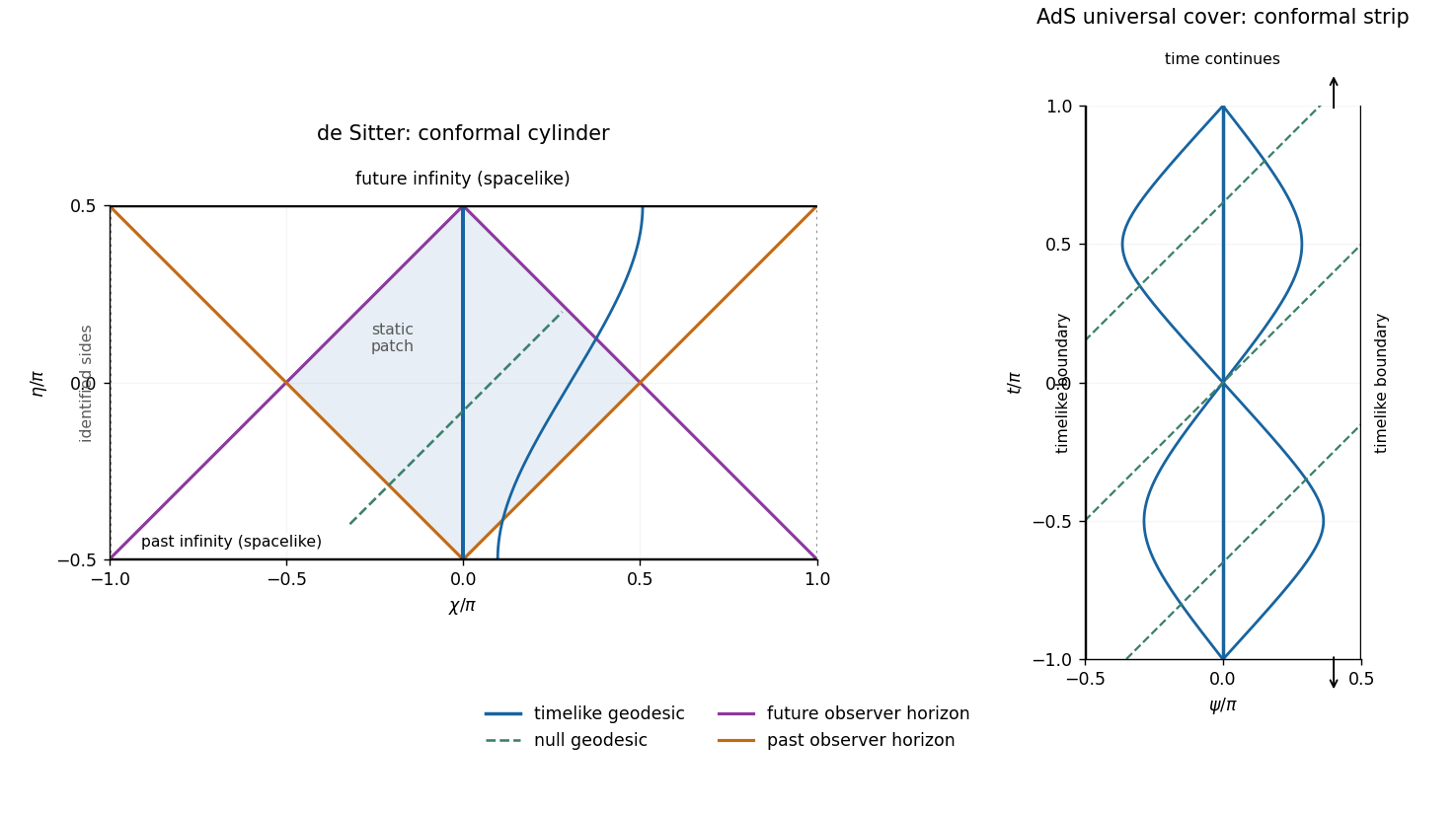
Conformal cylinder and observer horizons of two-dimensional de Sitter spacetime, compared with the timelike boundaries and geodesics of the AdS universal cover
. Details. 
The sides of the de Sitter diagram are identified; its top and bottom are spacelike infinities. The AdS diagram shows a finite window of an infinite time strip, with no identification of top and bottom. Null rays have slope one in both diagrams. The blue curves are timelike geodesics, while the colored de Sitter lines bound the central observer's causal domains.
The geodesics of two-dimensional de Sitter spacetime can be derived directly. Let an overdot denote an affine parameter normalized so that the tangent norm is for timelike, null and spacelike geodesics. The cyclic coordinate gives conserved , and normalization givesWriting reduces this to . For a future-directed timelike geodesic,The spatially comoving curves are geodesics, and every timelike geodesic extends through all , with infinite proper time in both directions. Initially comoving nearby observers have physical separation proportional to , displaying de Sitter's tidal defocusing. Relative separation can initially decrease for other initial velocities; not every pair is monotonically separating.
For a nontrivial null geodesic, and . Hence the conformal infinities at occur at infinite affine parameter, despite their finite values of . For a spacelike geodesic, and . Over a full affine-length period , integrating gives a change . Thus the spacelike geodesics close on the usual cylinder. The special case is the equatorial circle . These closed spacelike curves do not threaten causality.
The geodesics of two-dimensional anti-de Sitter spacetime instead conserve . Their norm equation givesA future timelike geodesic has andIts turning points are . Timelike geodesics oscillate rather than escaping to the spatial boundary. For , the central curve is geodesic. Integrating shows that a full proper-time period advances coordinate time by . They close on the periodically identified hyperboloid but remain complete nonclosed curves on the universal cover. Geodesics leaving reconverge at after proper time , illustrating AdS tidal focusing. A static observer at nonzero fixed is accelerated, not one of these oscillating free trajectories.
For AdS null geodesics, and . They approach either timelike conformal boundary at infinite affine parameter, while the coordinate-time travel from the centre is only . A spacelike geodesic has and connects the two spatial ends with infinite affine length. Both global models are geodesically complete. Reflecting a signal at the AdS conformal boundary is a choice of boundary condition for fields; it is not an automatic continuation of a geodesic at a finite affine endpoint.
For the complete de Sitter observer at , let be the shortest angular distance. An event at can send a signal reaching the observer at a finite future time exactly whenIt can receive a signal sent by the observer at a finite past time exactly when . Equality gives the future and past observer horizons in two-dimensional de Sitter spacetime; their null branches are respectively and on the displayed cylinder. Their intersection is the central static patch, . All complete timelike geodesic observers have analogous horizons by de Sitter symmetry. These are observer-dependent cosmological horizons, not singularities of the global coordinates or Cauchy horizons.
In contrast, the complete central AdS observer can exchange signals with every event at finite : the conformal distance is finite and the observer exists for all . Its static Killing vector has squared norm everywhere. Thus global AdS on its cover has no cosmological event horizon for this observer, although other restricted patches or accelerated observers can have horizons.
The causal predictability distinction is also important. Global de Sitter is globally hyperbolic: constant- circles are Cauchy surfaces. A causal curve is monotone in and satisfies ; if it ended at finite , compactness of the spatial circle would allow an endpoint and extension. Hence an inextendible causal curve crosses every such slice once. AdS on the cover has no closed timelike curves, but it is not globally hyperbolic. For two central events at and , with , their causal diamond contains events at and arbitrarily large , so it is not compact. Initial data alone do not determine field evolution without conditions at the timelike conformal boundaries. de Sitter has spacelike conformal infinities and cosmological observer horizons; covered AdS has timelike conformal infinities and requires boundary data. The distinction between the AdS quadric and its universal cover is also explained in David Tong's general relativity lectures.
Articles by others on the same topic
There are currently no matching articles.