Put , , and take a compactly supported Lighthill stress tensor. The isotropic term in that tensor is : the Kronecker delta is implicit in the printed shorthand. Convolving the Lighthill acoustic analogy with the retarded acoustic Green function and integrating twice by parts in the source coordinates givesThe boundary terms vanish because of compact support. For source size , the acoustic compact-source approximation requires . At , we may therefore replace the denominator by and the retarded argument by in the leading source integral. Define . In the radiation region , the leading two spatial derivatives act on the retarded time rather than on or :Thus the leading acoustic quadrupole density isFor the compact acoustic quadrupole Mach-number scaling, let be the source fluctuation speed, , and use the advective source time . With , one has and . ConsequentlyThe fourth power refers to the radiation coefficient with geometric spreading separated. It assumes that the source frequency scales as ; an independently imposed frequency or an independently strong thermal source would change that Mach number estimate.
Use time dependence and write the outgoing two-dimensional Helmholtz equation kernel as , where is independent of the Mach number. The harmonic Lighthill acoustic analogy givesFor a compact acoustic quadrupole, the source integral is . In the radiation region each derivative of the outgoing exponential supplies a factor of , soKeeping the same advective source-frequency scaling as in (i), and hence . Therefore the two-dimensional compact quadrupole scaling isThe changed exponent comes from cylindrical spreading . Compactness and the far-field condition are separate assumptions. At fixed imposed and fixed , with only varied, the stress instead gives an dependence; monochromaticity alone does not supply the additional source-frequency assumption.
Let , so the Lighthill stress tensor is . Write and . The distributional derivative of the Heaviside step function gives . Applying the product rule a second time yields the surface sources of a discontinuous Lighthill stress tensor:Repeated indices are summed. The first line gives the two bulk acoustic quadrupole distributions. The second line consists of additional surface delta distributions and their derivatives, all supported on the shock wave . For a symmetric Lighthill stress tensor, the first two coefficients of combine to after relabelling indices.
A discontinuity therefore adds both a surface-delta source and a surface-delta-derivative source. The level function need not be a signed distance: retaining its derivatives makes the expression invariant under a smooth reparametrization of the same surface. If the two bulk fields are only continuously differentiable, their second derivatives in the first line are read weakly; no classical second derivative is being assumed. The coefficients multiplying are kept as extensions, not replaced prematurely by traces.
Use the jump convention , consistent with region 1 occupying . The one-dimensional Lighthill stress tensor is , so . Both bulk stresses are constant. The distributional jump formula for a Heaviside product therefore givesThe Rankine-Hugoniot condition for conservation of mass is , while conservation of momentum gives . Hence a physical moving shock wave also satisfiesThis sign can be checked directly. Subtracting a constant reference density does not affect derivatives, and . Thus and , exactly reproducing the coefficient above.
Take , put and , and suppress the common factor . The upper-half-plane incident acoustic plane wave is . A rigid zero-thickness screen imposes the same normal-derivative cancellation on both faces; the scattered velocity potential is consequently odd in . Across the open part it is continuous, so its trace there is zero. These complementary half-line data are what make the Wiener-Hopf method applicable.
Use the Fourier transform , with inverse exponential . The outgoing Helmholtz equation solution is for , where has on the propagating interval and positive real part on evanescent components. The limiting absorption principle supplies the contour prescription. The transform of the trace supported on is analytic below the contour. Let be the analytic upper transform of the unknown derivative on . The prescribed derivative on has transformSince the upper normal derivative is , the Wiener-Hopf equation isFor the Wiener-Hopf factorization, choose analytic above and analytic below. Their branch cuts go into the opposite half-planes, with . Dividing by and performing pole subtraction in a Wiener-Hopf equation givesThe forcing pole is allocated to the lower analytic part; the second quotient has a removable pole and is upper analytic. Subtracting these parts leaves a common entire function. The finite-energy edge condition excludes an inverse-square-root singularity in the potential: its odd scattered trace is , so . The normal derivative on the open side can be , giving . Both sides of the entire remainder tend to zero. The Liouville theorem sets that remainder to zero, giving the explicit Wiener-Hopf solution of rigid half-plane diffraction:The scattered field on either side of the screen is thereforeIts forcing-pole residue at is . Deforming to the outgoing steepest descent contour crosses this pole precisely when , where , and . The residue contributes . Thus, away from transition boundaries, the scattered geometrical optics field isAdding the incident acoustic plane wave gives incident plus unit specular reflection in the upper reflected sector, just the incident wave in the remaining illuminated sectors, and zero in the lower shadow sector. The geometrical shadow boundaries also follow directly by tracing a straight ray to : the reflected ray hits the screen at , and the transmitted incident ray crosses the open part at .
For the diffracted contribution, the outgoing phase has saddle , value , and second derivative . Stationary phase therefore supplies . Substituting , and using , givesThe full asymptotic scattered field is . The angular edge-wave expression is not uniform on the geometrical boundaries. There is also a sign inconsistency in the supplied saddle formula: with its printed inverse exponential , the outgoing saddle is , not . The consistent inverse convention used above gives the requested outgoing field without that ambiguity.
Take a cut-on mode with , put and , so , , and initially take . The acoustic waveguide mode splits into two acoustic plane waves:At the upper edge , the upward-going constituent is incident from below. Use the reflected local coordinate ; its incident potential becomes , with local incidence angle . At the lower edge use and the downward-going constituent; it has the same local incident amplitude and incidence angle. At each wall the other constituent is the geometrical optics reflection of this incident half-amplitude, so it must not be counted again as an independent incident wave at the same edge.
Let . For a far observer, the upper and lower local observation angles are and , and their distances are and . Applying the Wiener-Hopf solution of rigid half-plane diffraction separately givesThe sign difference is the reversal of the upper-edge transverse coordinate. Their sum is the leading independent-edge radiation from an open planar duct:Restore if a time-dependent potential is desired. This is the leading large- approximation, neglecting further diffraction between edges, and assumes a far-field distance as well as . It is not a uniform approximation for a mode approaching cutoff. The zero mode follows as the grazing-incidence limit ; its beam-direction limit is treated separately below.
For , . Hence the numerator and denominator of the combined independent-edge radiation from an open planar duct both vanish at . At the positive angle, the ratio has the removable limitAt the negative angle the ratio changes sign, as does , so both directions give the same total velocity potential. Since , the result isFor the zero mode, use directly: . Its two directions coincide andThe two-edge field is finite in the constituent propagation directions. Its magnitude there is enhanced by a factor of order over an ordinary isolated-edge diffracted amplitude away from a shadow boundary. An isolated-edge angular formula has a pole in these directions, because its geometrical optics and edge-wave split is nonuniform; the exact single-edge field is not infinite. In the combined field the equal and opposite pole residues cancel, and the difference of endpoint propagation phases produces the finite limit above. Taking this combined limit describes the leading far-field beam; it does not justify evaluating either nonuniform single-edge expression separately at its pole.
Introduce , , and write . The method of multiple scales gives . At order , the resonant forcing is , because multiplication by generates only a constant and second harmonics. The solvability condition in the method of multiple scales therefore gives . A nonresonant particular correction isAt order , the forcing is . Its coefficient is . Removing this secular term givesPut , so . The slow amplitudes for the second Mathieu instability tongue satisfyThe initial conditions here are at leading order; a homogeneous correction makes the original data exact without changing . For example its initial cosine coefficient is in the chosen gauge. The slow squared growth rate is . Thus the robust leading stable ranges areSet in those ranges. The required explicit leading solution isThe remainder is uniform for , with fixed and fixed away from a changing instability edge. Inside , put ; replace the slow cosine and by and . The initial data excite this growing solution, so the leading solution is unstable.
At the leading endpoints the slow matrix is degenerate. Its continuous limits give at , and for these particular initial data at ; generic initial phases at the latter endpoint have slow algebraic growth. These are leading, not exact, instability edges. To specify the exact small- endpoint status, put , so the Mathieu equation has characteristic parameter and coupling . In the orthonormal cosine basis , the matrix has diagonal and adjacent couplings ; in the sine basis , the diagonal is and adjacent couplings are . Expanding the roots near of their determinants yieldsThese truncations determine the displayed orders because reaching the next omitted mode and returning requires at least six coupling steps. The fourth-order edges of the second Mathieu instability tongue are thereforeFloquet theory gives the unstable gap near this resonance. In particular, both fixed values and lie outside the exact gap for sufficiently small nonzero . Their fixed- solutions are bounded, although the leading slow matrix alone does not show this and the amplification bound is not uniform as .
Use and the WKB approximationAt leading order, the divergence-form acoustic Helmholtz equation becomes . The sloping-wall Neumann boundary condition becomes at . In the even transverse family this has normal modes , where , andFor the right-going propagating branch take real positive . The displayed local expression in the question must be read as a frozen-coefficient shorthand: the actual slowly varying phase is . Differentiating would instead give the erroneous local wavenumber .
The symmetric duct also has odd transverse normal modes . The integer-cosine form selects the even family requested here, rather than representing every duct mode. The approximation requires smooth slow variation and a positive separated from cutoff; it fails in a cutoff transition.
Let , , and . At the next order of the WKB approximation, the transverse operator givesThe moving-wall Neumann boundary condition gives and . Multiply by and integrate across the duct. Since and at both walls, integration by parts givesAlso , because at both walls. Substituting these identities in the next-order equation produces the transport equation for the variable-sound-speed WKB duct amplitude:Consequently is a complex constant, including a constant phase. For , ; for , , with the factor two absorbed into the mode's arbitrary constant. ThusEquivalently,There is an independent flux check. The real-coefficient Helmholtz equation implies , and the wall condition gives zero normal flux. Hence the integrated longitudinal current is constant; at leading order it is . This agrees with the transport equation. The factor must be retained: using only would ignore the variable coefficient in the given divergence-form equation.
Write , , and denote the slow density and velocity field amplitudes by and . Acting on the rapid phase, gives , where . Spatial differentiation gives , while derivatives of the amplitudes and the mean shear flow are . The leading continuity equation and linearized Euler equations therefore becomeEliminating on the nonzero acoustic branch gives the acoustic eikonal equation in a shear flow:The mean-shear term is small here because ; retaining advection does not require retaining that gradient in the leading phase equation. The positive intrinsic-frequency acoustic dispersion relation is , with group velocity .
In a stationary wall boundary layer, horizontal homogeneity preserves and along a Hamiltonian ray-tracing equations trajectory. For a two-dimensional ray,Suppose increases from zero at the wall to a positive free-stream value. For a downstream-directed wave normal, , increasing decreases and . The wave normal bends towards the wall, and the ray becomes more nearly parallel to it. If reaches , then : the ray turns and returns towards the wall rather than reaching the free stream. With launch angle above the wall and free-stream Mach number , the escape condition isFor upstream-directed wave normals, , and increase through the layer; there is no such downstream turning barrier on this branch. A wavefront normal is parallel to , while the energy ray follows the group velocity: advection makes their directions different. In particular, a wall-normal wave normal with can still have a ray drifting downstream. The ordinary WKB method needs a local turning-point continuation at ; the ray sketch depicts that qualitative continuation.
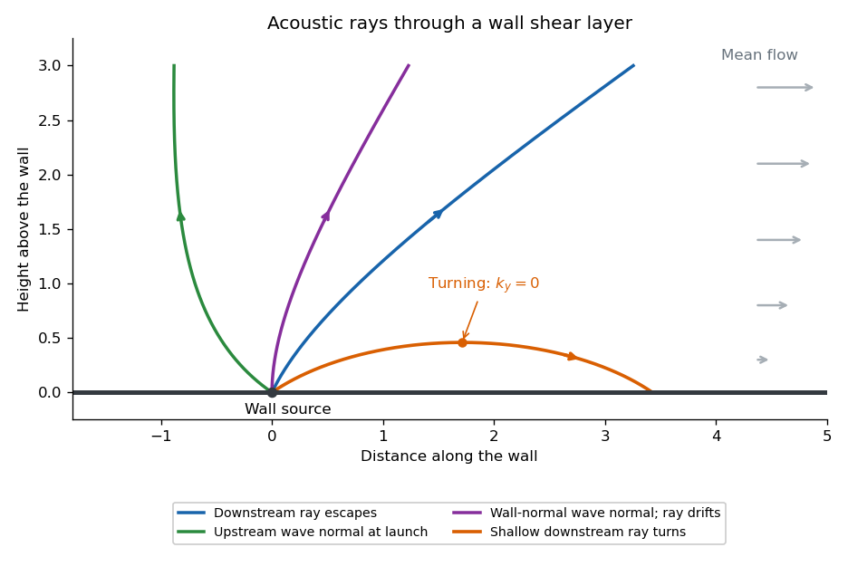
Acoustic energy rays through a wall shear layer, showing downstream escape, downstream turning and downstream drift of a wall-normal wave normal
. Details. 
For this sign of the viscous Burgers equation, the Cole-Hopf transformation is . Integrating the initial sinusoid gives ; the positive multiplicative constant cancels from . Set and . The Fourier series of the initial exponential and the heat equation yield the exact sinusoidal Cole-Hopf solution for negative-flux Burgers flow:Each harmonic decays by its heat multiplier, which can also be obtained directly by convolving it with the Gaussian heat-kernel convolution. At the first harmonic dominates:The error bounds use for real positive , also immediate from the Fourier-integral representation. Dividing, including the correction from the denominator, givesFor , the large-argument asymptotic expansion of a modified Bessel function gives . HenceThe sign is positive because the first Fourier harmonic of is negative, so its angular derivative is positive. For a fixed nonzero , the relative corrections vanish as and ; at the symmetry points both the exact solution and the leading expression vanish.
Put . For the Fay solution, . At the first harmonic therefore giveswhich agrees with the late-time limit in (i).
For the opposite limit, expand the reciprocal hyperbolic sine as a geometric series and interchange absolutely convergent sums at every :This exact positive-denominator form is useful near the shock. For small and , expand the denominator of the terms with small and use . The leading sum isFor the shock-layer scaling , the passage to this sum follows from dominated convergence: and for small provide a summable bound proportional to . The same leading expression matches the outer small-angle range . More generally, split the exact sum at with : the low terms have vanishing relative Taylor error, while the discarded exact and approximate tails are smaller than the leading expression by .
Now apply the partial-fraction identity for the hyperbolic tangent with :The Fay shock-layer asymptotics are thereforeThe angular shock thickness is , and its matched states are . At , both formulas vanish; the limiting slopes agree. The denominator throughout this derivation is as printed in the PDF, not the erroneous in the converted TeX.
Articles by others on the same topic
There are currently no matching articles.