Write for the reduced gravity. The Boussinesq approximation requires : replace density by in inertia and retain its difference in the gravitational force. A shallow-water approximation additionally requires a small aspect ratio, negligible leading-order normal acceleration and approximately hydrostatic pressure relative to the ambient fluid:Incompressibility makes the normal velocity smaller than the downslope velocity by the aspect ratio.
Thinness alone does not force the downslope velocity to be uniform across the layer. The additional top-hat plume model assumes that turbulent mixing makes both and approximately uniform inside it, with a sharp transition to the ambient fluid. Then the depth-integrated volume and momentum fluxes are and . This is the same integral closure used for a turbulent plume, applied to a shallow layer; the hydrostatic pressure term is retained because gravity has a component normal to the channel.
Assume the ambient fluid has zero downslope velocity, no bed drag, and an entrainment coefficient . The entraining shallow-water layer receives volume at rate , but neither excess buoyancy nor downslope momentum from that ambient fluid. Consequently volume conservation, conservation of excess buoyancy, and momentum conservation giveThe pressure contribution is the integral of the hydrostatic pressure from part (a). The last source is the downslope component of the gravitational force.
With , the equivalent equations areThe last term is the momentum required to accelerate newly entrained fluid. For variables , the matrix of the spatial derivatives isThus it is a strictly hyperbolic system for and . At all three characteristic speeds coincide and the matrix is not diagonalizable. The exclusion of that angle presumes the physical range with : allowing an overhanging channel with would also destroy hyperbolicity.
For the steady positive-velocity branch, conservation of buoyancy flux gives . Substituting into the other two balances givesUse a power-law ansatz , . The entrainment balance forces and . The momentum powers are , and , so the nonzero inertial branch has . Therefore the constant-speed entraining gravity current on a slope isIts positive speed requires for . In the shallow, strictly hyperbolic range this meansThe same steady integral balances have a formal vertical-plume limit at , although their time-dependent system then loses strict hyperbolicity. At the lower threshold the assumed positive-flux, finite-speed solution fails.
The line source is singular: and the momentum flux tend to zero, but diverges as . Thus this is a downstream ideal-source solution, valid only far enough away that and the Boussinesq approximation and top-hat plume model hold. It does not describe the immediate source region.
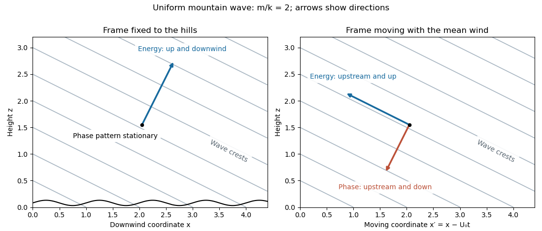
Take , , and represent the stationary topographic internal gravity wave by phase . Its laboratory angular frequency is zero, and its intrinsic frequency is . The internal gravity wave dispersion relation givesThe radiation condition selects , since this makes the vertical group velocity upward. The lower kinematic boundary condition is , so a corresponding linear wave field iswhere is the vertical fluid displacement. The constant-phase lines of an internal gravity wave slope down to the right, with .
Let . In the frame fixed to the hills the phase pattern is stationary: its phase velocity is zero, while the group velocity isEnergy travels up and downwind, with ray slope . In coordinates moving with the wind, the phase is . ThusThe intrinsic phase velocity is upstream and downward; the intrinsic group velocity is upstream and upward, perpendicular to the wave vector. Adding to the group velocity recovers the laboratory energy ray.
Vertically propagating waves require , equivalently . At equality the vertical group velocity vanishes; above the mountain-wave cutoff the bounded response is an evanescent wave. The linearization requires small terrain slope and small wave-induced displacement gradients , often summarized by . The model also neglects rotation, viscosity and compressibility; its scales must permit those approximations.
For a stationary component, the stationary internal-wave WKB solution has local vertical wavenumber and vertical-velocity amplitudewith the upward branch . The WKB approximation requires and sufficient smoothness, with a useful additional criterion. The background changes little over a vertical wavelength; this excludes a turning level of a stationary internal wave.
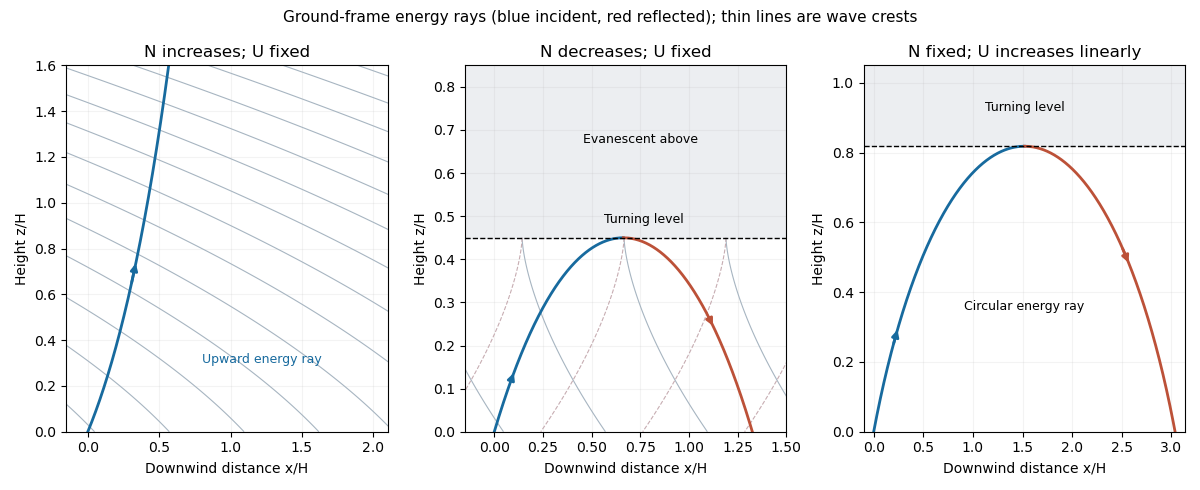
For increasing , the vertical wavenumber increases. The crest slope tends toward zero, and successive crests get closer vertically. The laboratory energy ray obeys , so it becomes more nearly vertical as it rises. There is no upper turning level in this ideal increasing-stratification profile.
For decreasing , the vertical wavenumber decreases to zero atThis assumes propagation at the bottom, . The crests become more nearly vertical and the incident energy ray becomes horizontal at . Above it the wave is evanescent, and the incident wave is reflected downward. The divergent WKB amplitude at is an approximation failure, resolved by an Airy function transition, rather than an infinite physical wave amplitude. The decreasing formula for is only a positive-frequency background below ; the relevant turning height lies below that level.


Let be pressure divided by the reference density and the buoyancy perturbation. The linear, inviscid Boussinesq equations about areFor a stationary Fourier component , incompressibility gives . The horizontal momentum equation then gives , while buoyancy conservation gives . Substitute these into the vertical momentum equation to obtain the stationary Taylor–Goldstein equation:Hence its local WKB approximation isFor negligible, an outgoing upward wave has . In particular for . In an upper evanescent region choose the branch with in so the solution decays upward. These choices express the radiation condition; a reflected wave has the opposite real branch and downward group velocity.
There are two different limiting levels. A critical layer in a shear flow occurs at , where the intrinsic frequency vanishes, , and upward propagation slows while the vertical wavelength contracts. Dissipation or nonlinear effects can absorb the wave and transfer its momentum to the mean flow. For a stable, slowly varying critical layer with Richardson number , the usual causal inviscid continuation suppresses transmission; it is not the same as reflection at . When the Richardson number is small, a general absorption-only conclusion needs extra stability assumptions.
Reflection instead occurs at the turning level of a stationary internal wave , beyond which . It is sometimes called a critical reflection height, but the wind there is nonzero. Assuming , the specified profiles giveThe decreasing-wind profile never encounters before its zero-wind layer. Both profiles have ; a well-separated WKB description requires , and a turning-layer transition is still required for the increasing profile.
The internal-wave ray tracing equations preserve the horizontal wavenumber and laboratory frequency. For the increasing wind, the upward branch satisfiesThe group-velocity ratio therefore givesIntegrating from yieldsThis is the ascending branch of the circular mountain-wave ray in linear shear:It reaches at , where the energy direction is horizontal. After reflection, and the ray continues downwind and downward along the other branchreturning to at . The last panel of the figure in part (b) shows this path. These are WKB energy rays, with the short neighborhood of the turning height supplied by its transition solution.
Treat the channel as prismatic, with horizontal bottom datum , uniform cross-sectional velocity, and surface height . The area and depth-integrated hydrostatic pressure force divided by density areThe prismatic-channel shallow water equations areSince , they becomeTheir two characteristic speeds are . Using gives the Riemann invariantsThe factor replaces the familiar for a rectangular channel. It comes from the depth-dependent width, not from a different gravitational acceleration.
For dilute sediment volume concentration , define . Neglecting particle volume in the fluid-volume balance,This applies the Boussinesq approximation to the bulk mixture, requiring , and uses a deep ambient layer . A gravity-current front condition closes the unresolved nose. Write it as , with a prescribed order-one front coefficient . If the chosen Froude number is instead , then .
Use a parabolic-channel sediment-current box model for one side of the dam: initially its length is , depth , and uniform concentration . Its conserved fluid volume isFor vertical settling onto the channel sides, the projected deposition width is . Thus the total particle deposition flux is andThe geometric factor follows from ; using a rectangular deposition formula would give a different result.
Eliminate time and use :The runout length of a gravity current is the limit where suspended concentration vanishes:The model approaches this length asymptotically in time. It assumes negligible entrainment, erosion and water loss, and does not resolve the initial release or nose. If the initially disturbed region supplies both sides, apply the formula to each side using its share of the initial volume and length.
For the early release, approximate the intact left half by water at rest at depth , and the right half by a dry bed. Put . The parabolic-channel dry-bed dam break is a centered rarefaction wave of the family, with the other Riemann invariant fixed at . Inside the fan, , soHenceThe left edge moves into the reservoir at and the dry front advances at . At the failed dam and . There is initially no finite-depth hydraulic bore into the dry bed: the depth falls continuously to zero.
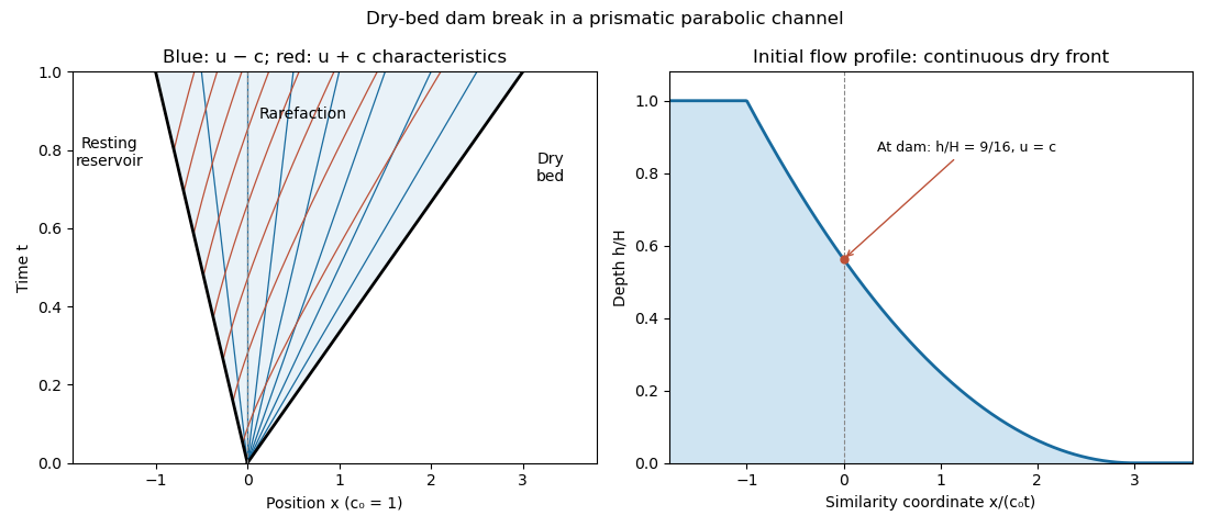
Characteristics and depth profile of the initial dry-bed dam break in a parabolic channel
. Details. 
On the – diagram, the characteristic curves inside the fan are straight rays from the origin. The curves obey , so they have form . The solution describes the period before the finite lake ends and their reflected signals matter. Immediately after failure, near the dam and very near the thin nose, strong vertical acceleration can invalidate the shallow-water approximation. The outer fan becomes appropriate when the horizontal flow scale is large compared with its depth.
Let states and be just left and right of a hydraulic bore moving at speed , and let . Integrating the conservative prismatic-channel shallow water equations across it gives the Rankine-Hugoniot conditionEquivalently the discharge in the shock frame is common on the two sides,Thus, for unequal positive depths,Momentum is conserved through the bore in this ideal model, but mechanical energy is dissipated; an energy-conservation jump must not be imposed as well.
For a stationary bore with rightward flow, , , and the momentum jump must still hold. A compressive hydraulic jump has andThe characteristic curves approach the stationary bore from both sides: upstream flow is supercritical flow, while downstream flow is subcritical flow using the local wave speed . The family travels downstream on both sides. These characteristic directions accompany, rather than replace, the two stationary conservation jumps.
Let and . For a deep-water gravity wave, and the first-order velocity potential is . ThereforeRelative to mean parcel labels, integrate at fixed zeroth-order position to obtain the oscillatory fluid displacementThe Stokes drift is the period mean of the displacement correction to the first-order velocity field:Thus , in the direction of propagation. A parcel samples faster forward motion near the top of its orbit and weaker backward motion lower down. This is the leading second-order drift of small-steepness waves, , relative to the Eulerian mean velocity.
Choose the positive-frequency branch with , let , and write . The internal gravity wave dispersion relation is . The phase velocity and group velocity areThey are perpendicular: the phase advances normal to the crests while energy travels along them. For a general signed , the positive frequency is and the horizontal component of group velocity changes sign with .
If , there is no real wave vector satisfying this relation. For prescribed real horizontal wavenumber, , so a bounded boundary response is an evanescent wave, rather than a freely propagating plane wave.
For a single incompressible plane wave, internal-wave polarization gives . Its oscillatory displacement is parallel to and therefore also perpendicular to . Every spatial derivative of the plane-wave field is proportional to a component of , soThere is no leading Stokes drift for that single wave. The fluid parcels oscillate along straight lines within phase planes and never sample a spatial change of the wave along their displacement. This conclusion does not prohibit cross terms between different wave vectors.
Assume and impose upward group velocity in . The two positive-frequency components then have wave vectors and with . Equal lengths are automatic, and orthogonality gives . HenceThe given orthogonal-wave condition is therefore possible only at this forcing frequency. The upward radiation condition excludes the branch.
Use superposition with vertical amplitude in each component and internal-wave polarization:The two sets of crests have slopes and ; their energy propagates upward and outward at angles of , while their phases travel downward. Their interference makes fixed horizontal bands of vertical-velocity nodes, at , and horizontal-velocity nodes, at .
Put , . The first-order displacement relative to mean parcel labels isThe horizontal displacement correction vanishes identically, whileConsequently the formal cross-wave Stokes drift isIt has alternating downward and upward columns, no depth decay in this ideal infinite plane-wave field, and zero horizontal-period-averaged vertical transport. Each wave alone has zero drift; the interference terms create this result.
This calculation is a kinematic second-order consequence of the linear field, not a complete prediction of mean transport. In particular, an impermeable oscillating lower boundary cannot have that nonzero mean normal parcel velocity. Its first-order displacement is . Expanding the exact kinematic boundary condition on givesThis Eulerian mean velocity cancels the computed normal Stokes drift at the material boundary. Away from it, the second-order mean-flow and buoyancy equations must also be satisfied. Thus the alternating drift is a valid formal cross-wave effect, but treating it alone as persistent transport with zero Eulerian mean would be physically incomplete. A prescribed permeable boundary would require its own second-order flux specification instead.
Articles by others on the same topic
There are currently no matching articles.