Past exam of the mathematics course of the University of Cambridge / 2013 / iii / Paper 53 (Structure and Evolution of Stars)

Assume $K>0$ and a positive central mass density. For this polytrope of index one, the spherical hydrostatic pressure support equation becomesDifferentiate the second equation and use mass conservation. With $k^2=2\pi G/K$, this givesThe regular central solution, with $\rho (0)={\rho }_c$ and ${\rho }^{\prime }(0)=0$, isThis is also the index-one solution of the Lane-Emden equation. The mass density remains positive up to its first zero, so the free surface is at $kR=\pi$, givingTaking a later zero would include a region of negative mass density and would not describe a physical star.

Integrating the mass givesConsequentlyThe radius is independent of the central mass density, whereas the mass is proportional to it; this is the special polytropic mass-radius relation at index one.

A nonspherical configuration requires the vector form of hydrostatic equilibrium and the Poisson equation, rather than the spherical mass-coordinate equations:For the same index-one polytrope, hydrostatic balance inside the positive-density region gives $\Phi =C-2K\rho$. Thus its interior mass density must obey the Helmholtz equationA positive separated solution with the required boundary values isIts maximum is ${\rho }_c$ at the centre of the cube and it vanishes on every face. Its Laplacian is $-3{\pi }^2\rho /L^2$, so it satisfies the interior equations whenTogether with $P=K{\rho }^2$ and $\Phi =C-2K\rho$, this explicitly constructs the cubic polytropic interior.

The mass integral separates into three elementary sine integrals:ThereforeThis construction satisfies the equations inside the prescribed cube. It does not by itself establish the existence of an isolated self-gravitating star: the interior potential must also match the exterior vacuum field generated by that very mass density. That additional physical requirement is addressed in part (c).

The cubic construction is a formal interior solution, not an isolated stellar equilibrium. The problem is more basic than whether a cubic star would be stable: the cubic polytrope fails isolated gravitational matching.

For a direct corner-force obstruction for a cubic polytrope, examine the corner at the origin. Every first derivative of the sine-product mass density vanishes there, so $\Phi =C-2K\rho$ predicts $\nabla \Phi (0)=0$. But the actual Newtonian gravitational potential of a positive mass density confined to this cube hasand similarly for the other two components. The integral is finite and strictly negative because the mass density is positive throughout the interior. The physical gravitational field is continuous up to this boundary point, so it cannot match the zero gradient of the proposed interior potential. An additive constant in the potential cannot fix that disagreement. The counterexample to a global interpretation is therefore the very constructed mass density: it solves the local equations but not the global gravitational boundary problem.

A nonrotating isolated fluid supported by an isotropic barotropic pressure normally has a spherical equilibrium. Rotation, tides and magnetic stresses can produce smooth departures from sphericity, but none of these is included in the cubic model, and no rigid walls exist to support its faces and corners. Observationally, ordinary stellar photospheres are consistent with approximately spherical shapes, or with oblateness and tidal distortions where those effects matter; there is no basis for expecting sharply bounded cubic stars. Thus the theoretical obstruction and the expected observations agree.

Use the notation $I_{\nu }(\mu ,\tau )$ throughout, with optical depth increasing inward and $0<\mu \le 1$ for an outward ray. This removes the change in argument order used in the printed surface-intensity notation. Multiplying the radiative transfer equation by its integrating factor givesIntegrating from the surface to a deeper boundary $b$ yieldsFor a semi-infinite atmosphere with no exponentially growing homogeneous term, the boundary term vanishes as $b\to \infty$. The formal solution of the radiative transfer equation is thereforeThe usual deep-atmosphere boundary condition is necessary; a first-order differential equation alone does not fix the emerging specific intensity.

For a linear source function, the zeroth and first exponential moments give $I_{\nu }(\mu ,0)=a_0+a_1\mu$. Equivalently $I_{\nu }(\mu ,0)=S_{\nu }(\tau =\mu )$, the Eddington-Barbier relation. If the source rises inward, rays near the limb sample cooler, shallower layers, producing limb darkening.

For the finite polynomial, put $u=t/\mu$ and integrate each term. Repeated integration by parts gives ${\int }_0^{\infty }{u}^j{e}^{-u}du=j!$, so the polynomial source function moments for emergent intensity giveThe limiting grazing-ray specific intensity is $a_0$. If the displayed polynomial is only a local Taylor approximation to a more general source, this formula applies to that approximation and a source-function remainder also contributes; a finite local expansion is not automatically an exact description at every optical depth.

For a constant source in an overlying layer of optical thickness $\tau$, the radial ray has the exact transfer relationExpanding the exponentials gives the constant source transfer through a thin layer:This finite-layer result does not require the specific intensity below the layer to equal its source function. The sign of $S_{\nu }-I_{\nu }(1,\tau )$ already distinguishes emission from absorption.

An absorption line forms when a bound-bound transition increases opacity at selected frequencies. In a photosphere whose temperature decreases outward, optical depth of order one at the line frequency occurs higher than at a nearby continuum frequency. In an absorption-dominated region in local thermodynamic equilibrium, the source is the Planck function; the cooler line-forming layer then emits less specific intensity than the deeper continuum-forming layer. The result is a dark spectral feature. Scattering and departures from LTE modify the source, so this temperature-gradient picture is a useful mechanism rather than a universal identity for every line.

Two distinct situations can produce emission lines. First, a heated chromosphere has an outward temperature rise, so an optically thick line can sample gas hotter than the continuum photosphere beneath it. Secondly, a hot optically thin circumstellar envelope or stellar wind emits line photons through collisional excitation or recombination, with no comparably bright background along all rays; its added line flux can exceed the underlying continuum. Winds of hot luminous stars can also give a mixture of emission and absorption across a Doppler-broadened line profile. These examples explain the change in specific intensity through either an enhanced source function or additional emitting material.

The high luminosity-to-mass ratio makes radiative acceleration and atmospheric departures from the simple approximations important. For an illustrative fully ionized hydrogen-rich composition with electron-scattering opacity ${\kappa }_e\simeq 0.34\mathrm{c}{\mathrm{m}}^2{\mathrm{g}}^{-1}$, the stellar electron-scattering Eddington factor isThus electron scattering alone removes roughly half of the effective surface gravity. It is below the Eddington luminosity, so electron scattering alone does not prove that a hydrostatic atmosphere is impossible. Line opacity can provide substantially more radiative acceleration and can drive a stellar wind.

For a plane-parallel atmosphere, the geometrical condition is that the line-forming region be thin compared with the radius. In a simple isothermal photospheric estimate, the atmospheric scale height isThis is plane-parallel validity from pressure scale height. The mass and luminosity alone do not specify $R$ or the atmospheric temperature, so they cannot decide the geometry uniquely. For example, if $T_e=3\times 10^4\mathrm{K}$ and $\mu \simeq 0.62$, the luminosity relation gives $R\simeq 37R_{\odot }$ and $H/R\simeq 3\times 10^{-3}$. Plane-parallel geometry could then be adequate for deep weak photospheric lines. It would still fail for lines formed over an extended wind, and a cooler, more extended supergiant needs a separate geometrical assessment. This numerical example is conditional, not an additional datum about the stated star.

LTE requires collisions and local thermal processes to establish the relevant excitation and ionization populations at the local gas temperature. In the dilute outer layers of a luminous hot star, radiative transition rates can dominate collisions, and the radiation field arriving from other depths is not the local Planck function. A non-LTE stellar atmosphere should therefore use statistical equilibrium with radiative and collisional rates coupled to transfer. Deep layers may approach LTE, but surface ionization balances and abundance-sensitive spectral lines are particularly susceptible to departures. An LTE abundance can be systematically wrong even when a plane-parallel approximation is geometrically good.

A static atmosphere requires velocities to be negligible where the diagnostic lines form. Massive luminous stars commonly have line-driven outflows, so static models cannot represent wind-formed profiles or their mass density and velocity gradients. A hydrostatic approximation can still be useful below the sonic region if the chosen lines form there, provided radiative acceleration is included in the effective gravity. Large outflows call for spherical moving-atmosphere models rather than merely a changed abundance in a static model.

The three assumptions cannot be accepted on the quoted mass and luminosity alone. LTE is especially doubtful in the outer layers; wind-sensitive abundance diagnostics require non-LTE moving models, and geometry must be checked through atmospheric extension and line-formation depth. Reliable stellar chemical abundances should be supported by observed wind signatures, temperature and gravity constraints, and agreement between several suitable ionization stages or weak photospheric lines.

The supplied rate law gives a local logarithmic temperature sensitivity, evaluated at fixed number densities. Since $\eta \propto T^{-1/3}$,Thus a power law here describes the tangent logarithmic slope near the chosen temperature, not an exact power law over all temperatures. For the three reactions, the factors $A{Z}_i^2{Z}_j^2$ are $1/2$, $24$ and $192/7$, respectively. At $T_6=15$ the local temperature exponent of a thermonuclear reaction givesHence $\alpha \simeq 4$, $\beta \simeq 16$, $\gamma \simeq 16$ and $\gamma >\beta$. The larger reduced mass for reaction 34 produces the last inequality. Composition changes contribute separately to an evolving reaction rate; they are held fixed for this derivative.

For the effective proton-proton reaction network, let the event rates beThe factors of one half count identical pairs once. Event 11 consumes two protons and makes one deuteron; event 21 consumes a deuteron and a proton and makes helium-3; event 33 consumes two helium-3 nuclei and makes one helium-4 nucleus and two protons. Under the stipulated fast-capture approximation, event 34 consumes helium-3 and helium-4 and supplies one mass-seven nucleus, and event 17 consumes that lithium-7 nucleus and a proton and makes two helium-4 nuclei. ThereforeFor closure, ${\dot{n}}_7={\lambda }_{34}{n}_3{n}_4-{\lambda }_{17}{n}_1{n}_7$. The stoichiometry conserves $n_1+2n_2+3n_3+4n_4+7n_7$, the baryon number density at fixed volume. In particular the mass-seven capture produces two helium-4 nuclei, not one.

The beryllium-to-lithium step is electron capture. Eliminating beryllium assumes that its capture flux tracks its production on the slow evolutionary timescale. More generally one retains ${\dot{n}}_{\mathrm{Be}}=R_{34}-{\lambda }_e{n}_{\mathrm{Be}}$ and ${\dot{n}}_7={\lambda }_e{n}_{\mathrm{Be}}-R_{17}$; setting the former to zero gives the effective equation used above. Fast capture relative to slow evolution alone would not prove that lithium exceeds beryllium: if both reach steady state their ratio is $n_{\mathrm{Be}}/n_7={\lambda }_{17}{n}_1/{\lambda }_e$. The mass-seven abundance assertion is thus part of the stipulated schematic limit, not a consequence to impose on every detailed solar model.

The enormous separation between the one-second deuterium destruction time and the other stated timescales justifies deuterium quasi-equilibrium in proton-proton burning:Substitution givesThe approximation is to the rapidly adjusting intermediate abundance, not to the slow proton abundance.

Near the centre the helium-3 relaxation time is also short compared with solar age and with the timescale of significant hydrogen evolution. Put $A={\lambda }_{33}$, $B={\lambda }_{34}{n}_4$ and $C={\lambda }_{11}{n}_1^2/2$. For slowly varying background quantities, the stable positive root of $A{n}_3^2+B{n}_3-C=0$ gives the helium-3 equilibrium abundanceThe other root is negative and unphysical. The production-minus-destruction function decreases strictly with positive $n_3$, so this is the unique attracting equilibrium. For $n_3=n_{3e}+x$, with the background held fixed during relaxation,Dropping the quadratic perturbation term gives the helium-3 relaxation timeIf the equilibrium itself evolves slowly, an additional forcing term $-{\dot{n}}_{3e}$ appears; tracking is accurate when this drift is small over one relaxation time. The given central value $6\times 10^5$ years is much shorter than the roughly $4.6\times 10^9$-year age of the Sun.

To estimate the temperature for helium-3 freeze-out, take the cooler pp-I-dominated regime and keep the background proton mass density approximately fixed for this order-of-magnitude scaling. ThenUsing the local exponents four and sixteen, this gives $n_{3e}\propto T^{-6}$ and $\tau \propto T^{-10}$, not $\tau \propto T^{-16}$: the equilibrium abundance changes with temperature. Normalizing at the central temperature givesSetting this equal to solar age yieldsThis is the requested power-law estimate. The exponents were evaluated locally at the central temperature, so extrapolation over this large range is approximate. Keeping the supplied full exponential rate factors in the same fixed-density pp-I estimate giveswhich gives about $6.8\times 10^6\mathrm{K}$. Thus the robust scale is a few million kelvin, roughly six to seven million in these estimates. A unique precise solar transition temperature cannot be obtained from the given numbers without the mass density, composition and pp-II contribution as functions of radius.

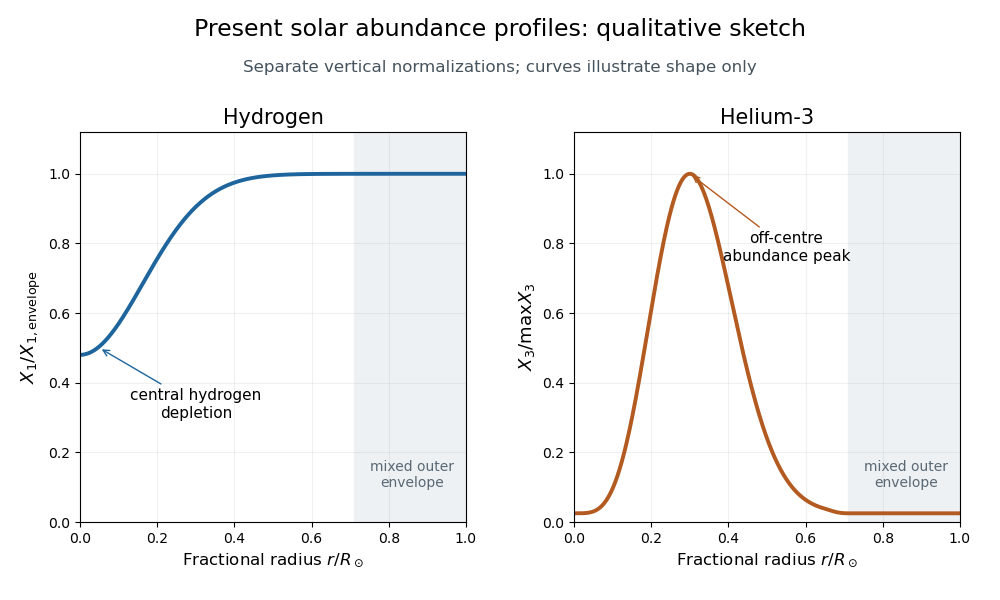
Finally, use mass fractions $X_i\simeq i{m}_u{n}_i/\rho$. The hydrogen mass fraction is depleted most strongly in the central burning region, so $X_1$ increases outward and approaches the nearly unprocessed envelope value. Convective mixing makes the outer envelope composition approximately uniform.

In the hot core helium-3 is quickly destroyed and remains close to its small equilibrium abundance. Moving outward, its destruction rates fall much faster than its production rate, so the equilibrium ratio $n_{3e}/n_1\propto T^{-6}$ rises. Where the relaxation time becomes comparable with solar age the abundance ceases to follow that rising equilibrium. Farther out, production itself becomes too slow to accumulate much helium-3, so $X_3$ falls again toward the envelope value. The result is a broad off-centre maximum, rather than a central maximum. These are the solar hydrogen and helium-3 abundance profiles requested by the sketch.

hydrogen rises from a depleted centre to an almost uniform envelope; helium-3 has a small central abundance and an off-centre peak before declining outward. The figure shows qualitative shapes with independently normalized vertical axes, not a fitted or computed solar model.