Past exam of the mathematics course of the University of Cambridge / 2013 / iii / Paper 66 (Biological Physics)

Take $A>0$ and use primes for spatial derivatives. Two integration by parts operations in the first variation of the elastic filament's bending energy giveThus the Euler-Lagrange equation is $A{h}^{\prime \prime \prime \prime }=0$, and the fluctuation differential operator is $K=A{d}^4/d{x}^4$. In the L2 space inner product, its boundary form isThe conjugate endpoint trace pairs are $(h,h^{\prime \prime \prime })$ and $(h^{\prime },h^{\prime \prime })$. Requiring one member of each pair to vanish gives the four standard self-adjoint endpoint conditions for filament bending, applied at both ends:

Each pair annihilates the boundary form for all $u,v$ in the domain. Conversely, the remaining two endpoint traces can be chosen freely: requiring the boundary form to vanish against every such $u$ forces an adjoint-domain function $v$ to satisfy the same two conditions. This proves self-adjointness, rather than just formal symmetry, on the corresponding fourth-order Sobolev space domain.

The count four concerns these elementary homogeneous choices. Identical-end boundary conditions do not restrict all self-adjoint operators to these four possibilities. For example, $h=0$, $h^{\prime \prime }=b{h}^{\prime }$ at both ends, with any fixed real $b\ne 0$, also annihilates the boundary form: the remaining expression is $-\overline{u^{\prime }}b{v}^{\prime }+b\overline{u^{\prime }}{v}^{\prime }=0$. This Robin boundary condition supplies a continuous family beyond the four listed pairs.

For each of the four standard pairs, integration by parts givesConsequently the eigenvalues are nonnegative. For a positive eigenvalue ${\mu }_n=A{k}_n^4$, the eigenvalue equation is $W_n^{\prime \prime \prime \prime }=k_n^4{W}_n$. Its four characteristic roots are $\pm k_n,\pm i{k}_n$, soHere $C_j$ are coefficients, avoiding a collision with the filament bending modulus $A$. The regular finite-interval self-adjoint operator has compact resolvent; applying the spectral theorem for compact self-adjoint operators to a shifted inverse supplies a complete orthonormal basis of eigenfunctions.

For clamped boundary conditions at zero, a clamped--clamped bending mode can be writtenAt $L$, writing $\beta =kL$, the two remaining boundary conditions areThe determinant is $2(1-\cos \beta \cosh \beta )$. Hence the positive wavenumbers obeyEquivalently, intersect $\cos \beta$ with $\mathrm{sech}\beta$. Numerical root bracketing givesThe entire sequence has the useful large-$n$ descriptionIndeed, put $\beta =(n+\frac{1}{2})\pi +\delta$ in $\cos \beta =\mathrm{sech}\beta$ and use $\cos \beta =(-1{)}^{n+1}\delta +O({\delta }^3)$ and $\mathrm{sech}\beta =2e^{-\beta }+O(e^{-3\beta })$.

The apparent root $\beta =0$ in the determinant equation is spurious for the clamped problem: at zero eigenvalue, $W$ is a cubic polynomial, and its four clamped conditions force $W=0$. For other endpoint choices, zero-energy filament modes must be treated separately from the trigonometric formula. The free-free kernel consists of affine functions, the torqued-torqued kernel consists of constants, and the hinged-hinged kernel is trivial. Including those kernels is necessary for a complete eigenfunction expansion.

Choose real eigenfunctions with ${\int }_0^L{W}_n{W}_{m}dx={\delta }_{nm}$. For positive modes, self-adjointness and integration by parts diagonalize the energy:At temperature $T$, the canonical ensemble is a product of centered Gaussian distributions. The equipartition theorem, with Boltzmann constant $k_B$, givesThe resulting thermal covariance of an elastic filament isFor an unnormalized eigenfunction of squared L2 norm $N_n$, divide its summand by $N_n$. This normalization factor cannot be absorbed silently into the modal variance.

For clamped boundary conditions at both ends, the inverse of $d^4/d{x}^4$ has Green function, for $x\le y$,It is cubic on each side of $y$, satisfies the four clamped conditions, has continuous first two derivatives, and has unit jump in its third derivative. Thus ${\partial }_x^{4}G=\delta (x-y)$, and its eigenfunction expansion is the sum above. In particular,These finite variances require removal of every zero-energy filament mode. An unconstrained free-free elastic filament can translate and tilt at no energy cost; a torqued-torqued elastic filament can translate. Their unrestricted Boltzmann distributions are not normalizable, so the full displacement variance is undefined. Fix those rigid degrees of freedom before applying the positive-mode formula.

For spatially varying tension in filament bending, keep the derivative of the filament tension as well as the curvature term. The first variation isTherefore the Euler-Lagrange equation and fluctuation operator areFor real, sufficiently smooth $\sigma$, the boundary form is the bending boundary form minus $[\sigma (\overline{u}{v}^{\prime }-\overline{u^{\prime }}v){]}_0^L$. Because $\sigma$ vanishes at both ends, the four self-adjoint endpoint conditions for filament bending still apply. The natural endpoint force also reduces there to the bending shear term. Thus $K_{\sigma }$ is a self-adjoint fourth-order scalar differential operator on the same chosen domain, with compact resolvent.

Choose a real orthonormal basis ${\psi }_n$ of eigenfunctions, $K_{\sigma }{\psi }_n={\lambda }_n{\psi }_n$, and write $h={\sum }_n{b}_n{\psi }_n$. Using the endpoint conditions in integration by parts givesThe equipartition theorem now gives, on the strictly positive subspace,This is a formal modal construction; no explicit eigenfunctions are needed. Nonnegative filament tension makes the energy nonnegative. Any surviving zero-energy filament modes must again be fixed. If signed $\sigma$ permits compression, self-adjointness still holds but does not guarantee a canonical ensemble: sufficiently strong compression can create negative eigenvalues and Euler buckling of an elastic filament. For instance, on $A=L=1$, take $\sigma =-Cx(1-x)$ and the clamped trial function $h=x^2(1-x{)}^2$. Thenso the energy is negative when $C>252$, despite $\sigma (0)=\sigma (1)=0$. The equipartition theorem requires a stable positive quadratic energy, not merely a real modal spectrum.

Use the homogeneous equilibrium point condition $k({\rho }_0){\rho }_0=a_{0}f({\rho }_0)$. Evaluate $D_1,D_2$ at $(a_0,{\rho }_0)$ and abbreviateThe quantity $c$ is the chemical relaxation rate with the cell density held fixed. Derivatives of $D_1,D_2$ do not enter this linear stability analysis: they multiply spatial derivatives of the homogeneous background or products of perturbations. For a Fourier mode with time dependence $e^{st}$, put $z=|\mathbf{q}{|}^2$ and writeConsequentlyAt $z=0$, the eigenvalues are $0$ and $-c$. The neutral cell-density mode reflects mass conservation, not decay of every homogeneous perturbation.

Write $a=D_2>0$, $b=D_{\rho }>0$, $C=D_1{f}_0$, and interpret production physically as $f_0\ge 0$. If $c\ge 0$, the trace-determinant stability criterion shows that an unstable nonzero wavenumber exists precisely when $C>ac$. The unstable band isIf $c<0$, the chemical field is already unstable at zero wavenumber; arbitrarily small positive wavenumbers are unstable too. Since $C\ge 0$, this also implies $C>ac$. Thus, on the infinite plane, the undivided Keller--Segel aggregation threshold isFor $\kappa >0$, dividing by $D_2\kappa$ gives the requested formAt equality there is no strictly growing mode when $c\ge 0$; nonzero spatial modes decay. On a finite domain, a permitted nonzero wavenumber must actually lie in the unstable band. If one allows a signed production function, the displayed matrix and trace-determinant stability criterion remain valid, but the simplification using $C\ge 0$ must be revisited.

The printed hypotheses do not ensure $\kappa >0$. Positivity of the degradation rate $k$ alone is insufficient. For a concrete counterexample, take $k(\rho )=e^{-2\rho }$, $f(\rho )=e^{-2}$, $a_0={\rho }_0=1$, and $D_1=D_2=D_{\rho }=1$. The homogeneous equilibrium point condition holds, all rates and transport coefficients are positive, but $\kappa =c=-e^{-2}$. The printed left-hand side equals $-1$, although $\det M=z(z-2e^{-2})<0$ for $0<z<2e^{-2}$. These spatial modes grow. If $\kappa =0$, the printed expression is undefined. The undivided criterion and the matrix above resolve both cases.

To find the fastest-growing Keller--Segel mode, use the larger eigenvalueFor $C>0$ the square root is real. Put $p=a+b$ and $d=b-a$. Differentiation givesA positive maximizing wavenumber exists in either of two growing cases: $c\ge 0$, $C>ac$, or $c<0$, $C>-bc$. Equivalently, $C>\max (ac,-bc)$. In this range $C+dc>0$, andThus the stationary point is the unique maximum. The derivative condition yieldsSolving it, with the root that satisfies the unsquared derivative equation, givesFor $c=0$, the unequal-diffusivity expression simplifies to $z_{\ast }=C/[\sqrt{ab}(\sqrt{a}+\sqrt{b}{)}^2]$, also agreeing with the equal-diffusivity limit. The formula maximizes the full two-field growth rate; it makes no instantaneous-chemical approximation. Every direction of $\mathbf{q}$ with this length is equivalent by rotational symmetry.

If $c<0$ but $0\le C\le -bc$, the maximum instead occurs at $z=0$: the fastest mode is homogeneous, with $s_{\ast }=-c$ and infinite wavelength. For $C>0$, its initial derivative is $-b+C/(-c)\le 0$. If $C+dc\ge 0$ the derivative thereafter decreases, while if $C+dc<0$ it increases towards the still-negative large-$z$ limit; either way no positive-$z$ maximum is missed. At $C=0$, the two eigenvalues are simply $-az$ and $-c-bz$, giving the same conclusion. In a finite box, maximize $s_{+}$ over the allowed Fourier modes; excluding the homogeneous mode can change the selected length. In a stable parameter range there is no fastest-growing mode.

The first ratio compares the positive feedback loop “more cells produce more attractant, which draws in more cells” with spreading by cell diffusion and removal of chemical perturbations. Its numerator $D_1{f}_0$ measures chemotaxis together with attractant production; its denominator $D_2\kappa$ measures dispersal together with incremental degradation. This competition between directed chemotaxis and cell diffusion produces spatial aggregation. The second ratio compares the concentration dependence of chemical production, $a_0{f}_0^{\prime }$, with incremental degradation $\kappa$. Positive $f_0^{\prime }$ amplifies chemical fluctuations, whereas negative $f_0^{\prime }$ suppresses them. It changes the chemical relaxation available to the chemotaxis feedback loop and can itself destabilize the homogeneous chemical field. Chemical diffusion $D_{\rho }$ suppresses short scales and sets the selected wavelength, but does not change the infinite-plane long-wave threshold. These interpretations as ratios of stabilizing and destabilizing processes assume $\kappa >0$.

Assume $D_0,n_0,Q>0$. The density-dependent diffusion coefficient makes this a cubic porous medium equation, since its two-dimensional form is $n_t=[D_0/(3n_0^2)]\Delta (n^3)$. The mass-preserving similarity solution is a radial cubic-diffusion source profile. At fixed $r$, the proposed scaled density givesSeparation is possible whenwhere $\gamma$ is a constant. The resulting ordinary differential equation isRecognize the second term as $\gamma ({\xi }^{2}F{)}^{\prime }$. Regularity and zero radial flux at the origin set the integration constant to zero:In the region $F>0$, this reduces to $F{F}^{\prime }=-\gamma \xi$, giving $F^2=1-\gamma {\xi }^2$ from the central normalization. For a nonnegative profile whose front is precisely at $\xi =1$, the first zero fixes $\gamma =1$. Continuity of the density excludes truncating a positive value at the front. HenceHere integrating the scale equation gives ${\lambda }^6=6D_{0}t/r_0^2+\text{constant}$, and the point-source initial condition requires $\lambda (0)=0$.

Use the planar area element, not the one-dimensional area under the drawn profile. Mass conservation givesThus the scale and the complete density arewhere $[u{]}_{+}=\max (u,0)$. The factors of $n_0$ are necessary on dimensional grounds; the length scale is not a function of $Q$ alone.

The front and peak obeyEach radial profile starts with horizontal tangent at the origin, decreases to a square-root edge, and is identically zero beyond $R(t)$. Later profiles are wider and lower. This is finite propagation in porous-medium diffusion, because the diffusion coefficient vanishes at zero density. The sketch uses dimensionless time $\tau =6D_{0}t/r_0^2$; it preserves the radial integral $2\pi \int rndr$, not the unweighted area under each curve.

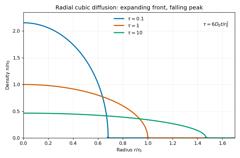
At the front $F^{\prime }$ diverges, so the profile is a weak solution, not a globally smooth classical solution. Nevertheless $F^2{F}^{\prime }=-\xi \sqrt{1-{\xi }^2}$ tends to zero there. The density and flux both match their zero exterior values, so extending the interior solution by zero creates no spurious boundary source in the conservation law. The behavior at the origin is regular because $F^{\prime }(0)=0$.

Finally, the point release is recovered as a distributional initial condition. For any continuous compactly supported test function $\phi$ on the plane, the total density remains $Q$ and all its support lies in the shrinking disk $r\le R(t)$. ThereforeThus $n(\cdot ,t)\to Q{\delta }^{(2)}$ as $t\downarrow 0$, in the sense of the Dirac delta function.