One convention for the Papkovich–Neuber representation uses a harmonic vector potential and a harmonic scalar potential :These are harmonic functions away from any singular force point. Since , the representation gives and , the equations of homogeneous Stokes flow.
Place the point force at the origin. A velocity linear in , decaying as and having the rotational symmetry of a point force is obtained from , . The vector components are harmonic functions for ; scalar dipole potentials would instead generate higher-order decaying singularities. The force normalization fixes . Indeed, substitution gives the Stokeslet:To verify its strength, the Newtonian fluid stress tensor is . Its outward traction integrated over any sphere surrounding the origin is , because . Thus the localized force applied to the fluid is , as required. Translation of the origin gives the same Stokeslet centered at any prescribed force point.
Let , , and letUse the method of reflections for Stokes flow. At the fixed sphere, the first sphere produces the incident Stokeslet velocity to leading order. In Faxén translation law, set the second sphere's translational velocity to zero. The applied holding force is thereforeThe first sphere's finite-radius potential dipole adds to the incident velocity, as does the Laplacian term in Faxén translation law at the fixed sphere. Multiplying by gives the stated next correction. There is no intermediate term. This is the holding force and torque for a sphere in a distant Stokeslet.
The vorticity of a Stokeslet at displacement is . At the fixed sphere, , soSet its angular velocity to zero in Faxén rotation law. The applied holding couple isThe displayed sign is the external couple needed to oppose the ambient rotation, rather than the hydrodynamic couple on the sphere.
The leading reflected flow at the first sphere is . Apply Faxén translation law there with its prescribed force . Since , the mobility correction from a fixed distant sphere isThe next correction comes from finite-radius terms in the incident/reflected flow and in Faxén translation law, together with the fixed sphere's induced stresslet and holding-couple rotlet. Each gives at the first sphere. The symbol is its isolated-sphere velocity scale, not its actual velocity in the two-sphere problem.
The first sphere has no applied couple. Its angular velocity follows from Faxén rotation law and the reflected Stokeslet:The component of parallel to contributes no vorticity. The next reflected rotlet and stresslet give the stated error order.
The mobility correction from a fixed distant sphere givesTaking their ratio and keeping the first nonzero transverse correction yieldsto the stated leading order. Set . The deflection is , so replacing by on the right introduces only higher-order errors. Integrating from givesThe maximum occurs at , and the deflection and spin in a distant sphere encounter areFor the rotation, use and to leading order in the angular velocity from part (b). Its signed angle about the positive axis isThus the rotation is clockwise when viewed from positive , with the magnitude of the displayed leading term.
The deflection tends back to zero downstream: . More generally, kinematic reversibility of Stokes flow combined with reflection in the plane makes a passing trajectory fore-aft symmetric. One can see this without using the distant-sphere approximation: the relevant translational hydrodynamic mobility matrix has the form . Hence is even in and is odd in . Uniqueness of the trajectory through then gives .
For , the numerical deflection and spin approximations above are invalid: the encounter enters a narrow gap and requires lubrication theory. However, the same return to the incoming offset holds for an ideal passing encounter of perfectly smooth spheres in Stokes flow. Lubrication resistance prevents finite-time contact under a bounded force, and does not itself destroy kinematic reversibility of Stokes flow. Contact, surface roughness or nonhydrodynamic forces could change that conclusion; they are additional physics, not part of the ideal model. This distinction is the fore-aft symmetry of a sedimenting-sphere encounter.
Take positive upwards and let denote axial body force per unit volume. With inertia and surface tension omitted, the extensional equations for a slender Newtonian column areMass conservation gives the first equation. The second uses the Trouton ratio three: the leading radial velocity is , the radial normal traction gives , and the axial stress is . An axial control volume balance then gives the displayed equation. The approximation requires a slender column and slowly varying radius.
Let . Since the container base is closed, the total volume flux at every section is zero. The column carries flux , so the annulus carries and has mean speed of order . Its interfacial shear stress is therefore of order . Transmitting this stress through the core produces an axial velocity variation of order . The plug-flow criterion for a column in a low-viscosity annulus is consequently
Use modified pressure , removing the annular fluid's hydrostatic pressure. In a local planar gap, with at the column and at the container wall, lubrication theory givesThe required return flux per unit circumference is to leading order in . Its pressure-driven component is larger than the Couette component by , so the annular return flow around a slumping column givesThe annular shear contribution to the integrated axial force is smaller than this pressure-gradient term by . Retaining the leading terms and substituting gives the dimensional equationsThe boundary conditions are at the base and at the free upper end; the latter expresses zero excess axial extensional stress.
For , defineThis function records the leading thin-annulus resistance; differences from curvature and the Couette term enter at the already neglected relative order . Choose the extensional screening length of a slumping column and the associated scales asHere denotes the initial annular gap in this question. With , and , the dimensional equations reduce to
Initially and , so , with and . The initial velocity profile of an annularly confined column isThe column thickens everywhere below its stress-free top, while that initial thickening rate is zero at the top.
For a tall column, , the limiting forms away from exponentially small end corrections areThe bulk falls at approximately , where excess weight balances annular hydraulic resistance. Extensional stresses adjust this velocity to zero in a basal boundary layer of thickness ; almost all thickening occurs there.
For a short column on this scale, , while still slender, the limits areThe annular-resistance term is small, so excess weight is balanced predominantly by extensional viscous stress. The top speed is , recovering the zero-annular-viscosity result. Thus is the vertical distance over which extensional stress communicates the basal constraint before annular resistance screens it. The sketches below use separate natural normalizations for the two limits.
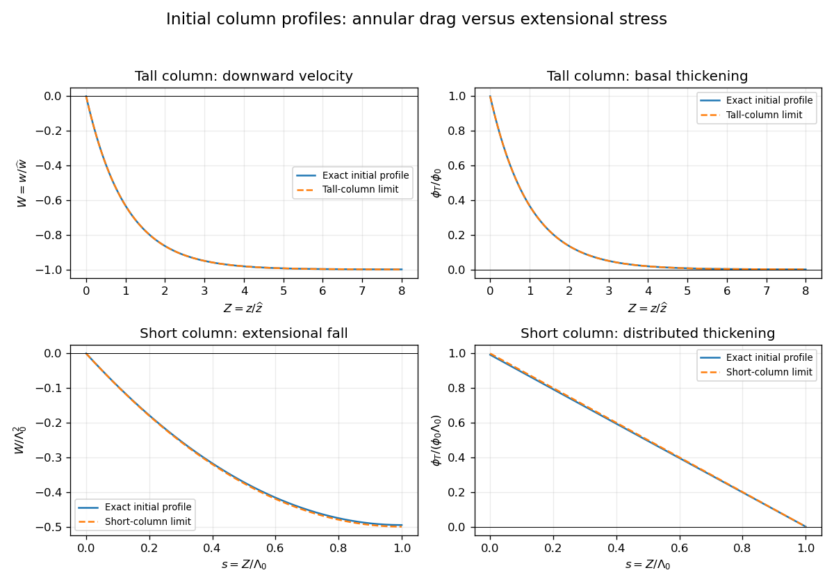
Initial velocity and thickening profiles of long and short annularly confined viscous columns
. Details. 
At leading order in the lubrication approximation, surface arclength is horizontal distance. An insoluble surfactant is transported by the surface velocity, without bulk exchange or diffusion. Conservation of insoluble surfactant on a moving interface therefore becomesThe local hydrostatic pressure and capillary normal stress giveSolve with no-slip boundary condition at and Marangoni stress . The velocity, surface velocity and volume flux per unit width areMass conservation, , yields the thin-film equations with insoluble surfactant:and the corresponding surfactant equation isThe hydrostatic and capillary terms thus affect both the film flux and the surface transport, with different coefficients.
For finite-mass Marangoni spreading on a liquid film, first neglect both pressure-gradient terms. If the spread has size , then and , giving surface speed . Equating to this speed givesSet exactly as a similarity scale, and writeOn the positive half of the pool, substitution produces two ordinary differential equations:Symmetry fixes the flux integration constant in the second equation to zero, giving wherever . Substitution into the first equation gives . Thus the linear similarity profiles for surfactant spreading have the formThe concentration vanishes at the moving front. The two integral constraints are total surfactant mass and conservation of the fluid volume relative to the undisturbed layer:The first gives ; the second gives . Therefore . In physical variables, the solution isOutside the pool the leading outer solution has , . In particular, : the subscript means the one-sided limit just behind the front. As a consistency check, the surface speed there is and the fluid jump satisfies the moving-front mass conservation condition. This ideal outer solution has a height jump from to .
That jump cannot persist in a physical interface with nonzero gravity or surface tension. Across a smoothing region of width , changes by . The Marangoni flux scales as . At , its balance with the capillary flux gives capillary smoothing of a Marangoni front:Here the surface tension approaches at the surfactant-free edge. The assumed concentration-gradient scale is even inside the smoothing region.
When gravity dominates capillarity, the hydrostatic flux is . The same balance gives gravity smoothing of a Marangoni front:The gravity-dominated condition is , the square of the capillary length. The printed condition omits ; the expression above restores dimensional consistency.
This width grows faster than . It becomes comparable with the pool size whenThe time is a scaling estimate, so numerical factors cannot be fixed by the width balance. For , the sharp-front similarity profile no longer describes the film: hydrostatic pressure levels the layer over the whole pool, and its thickness tends towards with an increasingly small depression beneath the surfactant. The surface can still spread by Marangoni stress while a hydrostatic-pressure-driven return flow nearly cancels the net film flux. In this gravity-levelled surfactant film, gives , so the fractional height variation is of order .
Use pressure with the ambient hydrostatic pressure removed, and let be the pressure below the falling sphere minus that above it. Away from the sphere the tube flow is Hagen-Poiseuille flow. The upper and lower clear lengths add to to leading order in , so their pressure drops add:The large exterior reservoir returns this flux with negligible pressure loss compared with the long narrow tube. The sphere is assumed far enough from the ends that entrance effects and its occupied length give only lower-order corrections.
Now use a frame translating downwards with the sphere, and take positive upwards from its center. The sphere is stationary and the tube wall moves upwards with speed . The narrow gap isIt has axial length scale , making lubrication theory appropriate. The sphere-frame flux in a tube is constant: the upward relative flux through the whole section is , so its flux per unit circumference isWith on the sphere and on the wall, Couette-Poiseuille flow in a thin gap givesSince , the pressure-jump relation isThe parabolic inner gap can be extended to infinite because these integrals are dominated by . The lubrication resistance integrals for a nearly occluding sphere areSetting evaluates , , , hence
For the force, enclose the fluid between sections just above and below the sphere, including the annular layer. The net upward pressure force is . The tube wall exerts upward shear traction on this fluid; the sphere exerts a downward force equal to the upward hydrodynamic force on itself. From the gap solution,The axial control volume force balance therefore gives the control-volume drag formula for a sphere in a tube:Using a control volume avoids having to integrate the curved-sphere normal pressure and tangential shear separately.
With , , , , and , the three flux/pressure equations becomeSolving these linear relations givesThe force relation is . Substitution first yieldsBecause and , the terms and are lower order than . Keeping the uniformly relevant leading terms givesThe squared is essential; replacing it by would give the wrong sign and scaling. This establishes the three drag regimes for a nearly occluding sphere.
For ,The sphere nearly carries the tube's fluid down with it: the far-field flux is close to the piston displacement rate. The relative annular leakage is small in total volume, and the dominant force comes from the local annular shear term. The pressure force associated with the overall tube resistance is smaller.
For ,The flow remains approximately piston-like, but the dominant force is now the pressure needed to drive Hagen-Poiseuille flow through the long clear tube. Both displayed terms in are retained because their relative size changes inside this regime without producing an additional leading drag regime.
For ,The large tube resistance makes its net through-flow negligible. The sphere's displaced fluid instead passes upwards relative to it through the thin annular gap, with gap velocity of order . Its pressure drop and resulting pressure force dominate.
Finally consider two identical co-moving spheres, with nonoverlapping lubrication regions and the same total clear-tube length to leading order. The common through-flux is not doubled. In the middle regime it is still approximately , so the same total tube pressure drop is shared equally between the two identical spheres. The load sharing between co-moving spheres in a tube gives half the single-sphere force on each sphere in regime (ii). In regime (i), drag is set locally by the nearly pressure-balanced annular shear and is unchanged on each sphere. In regime (iii), each sphere must pass essentially its own displacement flux through its annular gap, giving the same local pressure drag as before; adding another pressure jump changes the already small tube flux but not either leading drag. The force is unchanged in regimes (i) and (iii).
Articles by others on the same topic
There are currently no matching articles.