Past exam of the mathematics course of the year 1 of the natural sciences course of the University of Cambridge / 2004 / Paper 2

Choose a common origin at vertex $C$, set $\mathbf{a}=\overrightarrow{CB}$ and $\mathbf{b}=\overrightarrow{CA}$, and orient the remaining edge as $\mathbf{c}=\overrightarrow{AB}$. ThenThis convention makes the interior angle between $\mathbf{a}$ and $\mathbf{b}$ equal to $C$, and their lengths equal to the opposite side lengths $a$ and $b$.

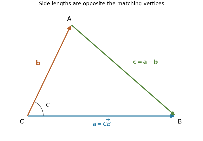
Take the dot product of the difference with itself. Since $\mathbf{a}\cdot \mathbf{b}=ab\cos C$, the law of cosines follows:The magnitude of the cross product of two edge vectors is twice the triangle's area $K$. Applying this at each vertex gives $2K=ab\sin C=bc\sin A=ca\sin B$. Divide by the nonzero product $abc$ to obtain the law of sines:

Let $\Omega$ be the interior of the tetrahedron, and take any constant vector field $\mathbf{q}$. Its divergence is zero, so the divergence theorem givesChoosing $\mathbf{q}$ to be each Cartesian basis vector proves ${\sum }_i{\mathbf{V}}_i=0$. This is the general fact that vector areas of a closed polyhedron sum to zero, specialized to four faces. The outward orientations are essential: the scalar face areas are all positive and do not sum to zero.

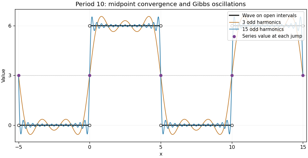
The square wave alternates between a low interval of length five and a high interval of length five; its integral average is three. In the real Fourier series conventionintegration over one period givesandThus only odd harmonics occur:The Dirichlet-Jordan convergence theorem makes the sum equal to the function at its continuity points and to the mean of its one-sided limits at a jump. Consequently the sum is 3 at each of $x=-5,0,5$, regardless of any separately assigned values of the original function at those endpoints.

For orthogonal matrices $Q_1,\dots ,Q_m$ of the same size, transpose reverses the order of multiplication. Thereforeby canceling the adjacent pairs $Q_j^T{Q}_j=I$ successively. Hence every finite product is an orthogonal matrix.

The given symmetric matrices satisfy $E_j^T{E}_j=E_j^2=I$, so both are orthogonal matrices. Put $J=E_1{E}_2$, $c=\cos (\theta /2)$ and $s=\sin (\theta /2)$. Anticommutation givesThus $A=cI+sJ$ and $A^T=cI-sJ$, giving $A{A}^T=(c^2+s^2)I=I$. These are orthogonal rotations generated by anticommuting involutions. Also $A-A^T=2sJ$. Since $J^2=-I$ makes $J$ invertible, $A$ is symmetric exactly when $\sin (\theta /2)=0$.

Use $J{E}_1=-E_2$, $E_{1}J=E_2$ and $J{E}_{1}J=E_1$ to expand the matrix product:The double-angle identities therefore giveSimilarly $J{E}_2=E_1$, $E_{2}J=-E_1$ and $J{E}_{2}J=E_2$, soThis conjugation rotates the two-dimensional span of the two matrices through the double angle described by orthogonal rotations generated by anticommuting involutions.

Write the general real symmetric matrix as $E_2=\left(\begin{array}{cc}r& t\\ t& u\end{array}\right)$. With the specified $E_1$, anticommutation readsHence $t=0$ and $u=-r$. The remaining condition $E_2^2=I$ gives $r^2=1$, leaving exactlyBoth matrices directly satisfy all the conditions.

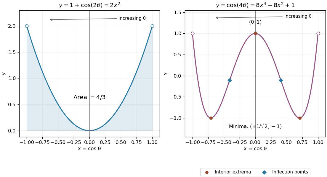
The double-angle identity eliminates the parameter: $y=1+\cos 2\theta =2{\cos }^2\theta =2x^2$. As $\theta$ increases from zero to $\pi$, $x$ decreases from one to minus one. The positive area below this parabola is thereforeEquivalently, the parameter integral is $-{\int }_0^{\pi }(1+\cos 2\theta )(-\sin \theta )d\theta$. The leading minus sign corrects for traversal from right to left; the signed integral $\int ydx$ along that traversal would be negative.

For $0<\theta <\pi$, the chain rule for a parametric curve givesAt $\theta =0$ the quotient of parameter derivatives is formally $0/0$, but the simplified expression has limit $16$. Thus the limiting tangent at $(x,y)=(1,1)$ has gradient 16. This is an endpoint limit of the given open parameter interval, or the ordinary tangent of the smooth polynomial extension $y=8x^4-8x^2+1$.

The fourth Chebyshev polynomial eliminates the parameter:Its derivatives are $y^{\prime }=16x(2x^2-1)$ and $y^{\prime \prime }=16(6x^2-1)$. The interior stationary points are a local maximum $(0,1)$ at $\theta =\pi /2$, and two minima $(\pm 1/\sqrt{2},-1)$ at $\theta =\pi /4,3\pi /4$. At the maximum $y^{\prime \prime }=-16<0$, while at either minimum $y^{\prime \prime }=32>0$.

The two inflection points areThe curvature changes sign there. The endpoint limits are $(\pm 1,1)$, at $\theta =0,\pi$; they are excluded from the open curve. The central maximum and the two minima are also the attained global extremal values on that open curve.

Use the intended model of independent Bernoulli trials, with the same scoring probability $p$ for every shot. Equal marginal scoring probabilities alone would not establish the stated formula without independence. Let $N_1,N_2$ count misses in the two groups of five. They are independent random variables with binomial distribution $\mathrm{Bin}(5,1-p)$. A tie occurs precisely when $N_1=N_2=n$ for one of the mutually exclusive possibilities $n=0,\dots ,5$. Therefore the tie probability for independent binomial counts isAt $p=1/2$, Vandermonde's identity gives ${\sum }_n{\left(\genfrac{}{}{0ex}{}{5}{n}\right)}^2=\left(\genfrac{}{}{0ex}{}{10}{5}\right)=252$, soExchanging the two teams preserves the distribution and interchanges the two winning events. Their total probability is $1-\alpha$, so the first team wins at the end of the initial period with probability $193/512$. In this model the shooting order gives no advantage.

Each additional pair of independent shots resolves the tie with probability $r=2p(1-p)$, since exactly one team must score. It preserves the tie with probability $q=p^2+(1-p{)}^2=1-r$. Finishing after $10+2k+2$ shots means an initial tie, then $k$ tied pairs, then a decisive pair. Independence and geometric continuation after an initial tie giveBecause $0<p<1$, $r>0$ and $q<1$. The total eventual winning probability is the sum of winning in the first ten shots and winning later:Equivalently, conditional on the initial tie, the probability of still being tied after $m$ further pairs is $q^m\to 0$.

For the negative-sign equation, take a nonzero separated solution $\varphi =X(x)Y(y)$. Separation of variables gives $X^{\prime \prime }=-\mu X$ and $Y^{\prime \prime }=-(25-\mu )Y$. The zero Dirichlet boundary conditions on $X$ force $\mu =m^2$ with a positive integer $m$ and $X=\sin mx$, up to a constant. Zero boundary values on $Y$ similarly require $25-m^2=n^2$ with a positive integer $n$. A zero or negative separation eigenvalue would give linear or hyperbolic factors, whose two zero endpoint values force the trivial solution.

The only positive integer pairs with $m^2+n^2=25$ are $(3,4)$ and $(4,3)$. By the complete Dirichlet eigensystem of a rectangle, these span the whole eigenspace, soFor the positive-sign equation there is only the zero solution. One can use the same strictly positive eigenvalues of $-\Delta$, or directly apply the zero Dirichlet solution of the modified Helmholtz equation. Multiplying by $\varphi$ and using Green's first identity giveswhere $\Omega =(0,\pi {)}^2$. Both nonnegative integrals must vanish, proving $\boxed{\varphi =0}$.

Set $H(x,y,z)=x^3+xy+yz-1$. The gradient $\nabla H=(3x^2+y,x+z,y)$ is a normal vector to its level set. Since $y\ge 1/2$ on the given patch, division by its last component is valid and gives the unique normalized fieldIts dot product with $\mathbf{k}$ is one, as required; it is not generally a unit vector.

Orthogonal projection of a small surface patch onto the $xy$ plane multiplies its scalar area by $\cos \alpha =\mathbf{n}\cdot \mathbf{k}>0$. Hence $dxdy=\cos \alpha dS$ and $d\mathbf{S}=\mathbf{n}dxdy/\cos \alpha$. Since $\mathbf{n}=\mathbf{u}/|\mathbf{u}|$ and $\mathbf{u}\cdot \mathbf{k}=1$, one has $\cos \alpha =1/|\mathbf{u}|$. The vector area element of an implicit surface is thusThe positive final component implements the specified upward orientation.

Take the dot product of the given field with the upward vector area element. The surface relation simplifies its integrand:The projected domain is exactly the rectangle $1/2\le x,y\le 1$, since $y>0$ determines a unique $z=(1-x^3)/y-x$. Therefore the surface integral is

The defining function $x^3+xy-1$ is independent of $z$, so a normal vector is $(3x^2+y,x,0)$. It never vanishes here because $x>0$. Every normal is horizontal, whereas $\mathbf{G}=(0,0,x)$ is vertical and tangent to the surface. Their dot product is zero at every point, givingThis is independent of orientation. Although the surface extends without a bound on $x$, the integrand vanishes identically, so no convergence problem arises for this flux.

Multiply the Taylor expansions $\ln (1+x)=x-x^2/2+x^3/3+O(x^4)$ and $(1-x{)}^{-1}=1+x+x^2+O(x^3)$. Collecting the first three nonzero coefficients givesThe cubic coefficient is $1-1/2+1/3=5/6$.

Use the geometric series $(1+u{)}^{-1}=1-u+u^2+O(u^3)$ with $u=\sin x=x+O(x^3)$. The constant term counts as the first nonzero term, so the requested expansion is

Write $\cos x=1+u$ with $u=-x^2/2+x^4/24-x^6/720+O(x^8)$. Substitution into $\ln (1+u)=u-u^2/2+u^3/3+O(u^4)$ givesThus the first three nonzero terms of this even Taylor series areThe real logarithm is well defined near zero because $\cos x>0$ there.

Multiply the two power series and collect equal powers of $x$. The Cauchy product givesOnly terms whose two exponents add to the target exponent contribute.

In the Cauchy product, $a_j{x}^j$ combines with $b_{i-j}{x}^{i-j}$ to give a term of degree $i$. HenceThis coefficient identity holds for formal power series. For convergent Taylor series it also gives the function product throughout the common open interval of convergence, where absolute convergence justifies regrouping.

The product rule and chain rule first giveDifferentiating the first expression with respect to $y$ yields $e^{x^{2}y}(2y+7x^2{y}^2+2x^4{y}^3)$; differentiating the second with respect to $x$ gives exactly the same polynomial factor. ThusThis also follows from symmetry of second derivatives, since all derivatives of this function are continuous everywhere.

Use the fixed exponents $p,q$ in the original PDF. Assume positive $a,b$ so arbitrary real powers and a relative change are defined. Set $h=k/100$. With $b$ fixed, the exact new-to-old ratio is $(1+h{)}^p$. The binomial series, or the one-variable case of the second-order relative change of a monomial, givesTherefore the approximate percentage change through second order isFor negative $k$ this same signed expression describes a decrease.

Set $h=k/100$ and $j=m/100$. The exact ratio is $(1+h{)}^p(1+j{)}^q$. Multiplying the two binomial series and retaining total degree at most two gives the second-order relative change of a monomial:Multiply by one hundred to express the change as a percentage:The cross term accounts for the simultaneous changes in both inputs and cannot be recovered by simply adding their separate second-order percentage changes.

The function $x^{-3}$ is strictly decreasing for positive $x$. On $a<x<a+1$, this gives $x^{-3}<a^{-3}<(x-1{)}^{-3}$. Integrate across that unit interval to obtainApplying this to every integer $n\ge a$ and summing proves the integral test tail boundsBoth remain strict: the sum of the positive differences between rectangles and integrals is already bounded below by its positive first difference. Convergence of the integrals and the p-series makes the passage to infinity valid.

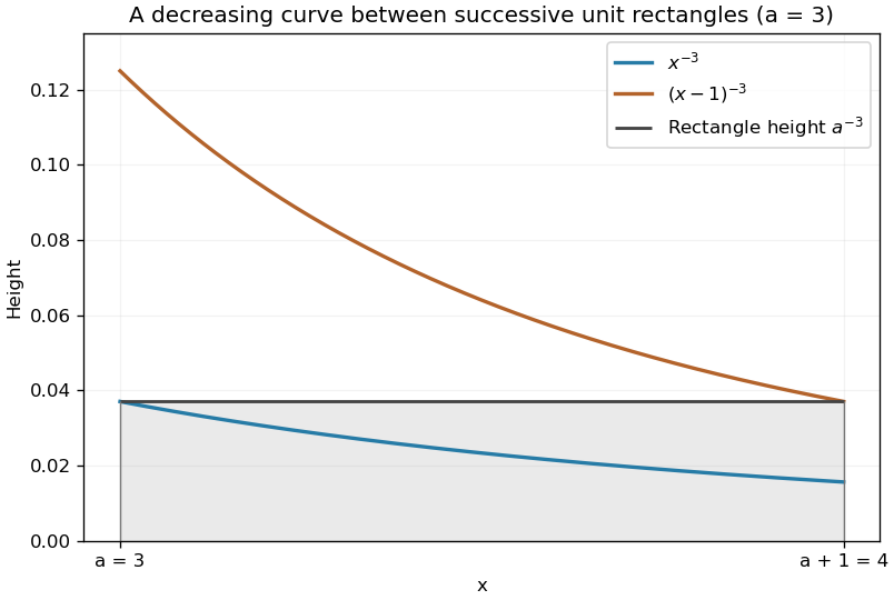
The shifted integral representation of a p-series tail evaluates the defining integral asIt is strictly increasing in $k$, since $I_p^{\prime }(k)=(5-k{)}^{-p}>0$. From the bounds just proved with $a=5$, $I_3(0)<{\sum }_{n=5}^{\infty }{n}^{-3}<I_3(1)$. Since the middle expression equals $I_3(k_3)$, monotonicity proves

Subtract the first four terms from the given full p-series sums. WriteandSolving $I_p(k_p)=S_p$ yields $k_p=5-[(p-1)S_p{]}^{-1/(p-1)}$. ThereforeThe unrounded shifts are approximately $0.4817158633$ and $0.4638861447$.

Use the stipulated interpolation $k_3\approx (k_2+k_4)/2$. The unrounded values give $k_3\approx 0.4728010040$, and henceThus a sensible reported estimate isUsing the rounded shifts from part (ii) instead gives $k_3\approx 0.473$ and a sum about $1.202059745$, with the same six-significant-figure estimate. The interpolation of shifts is an assumption of this approximation; the integral test bounds alone do not prove that many digits of accuracy.

For $x=e^z>0$, let $Y(z)=y(e^z)$. The chain rule givesMultiplying each original Cauchy-Euler equation by $x^2$ therefore givesandThe exponential change of variable has made both equations have constant coefficients.

For equation (1), the characteristic equation is $r^2+3r+2=(r+1)(r+2)=0$, so $y=A/x+B/x^2$. The initial conditions give $A+B=0$ and $-A-2B=1$, whence $A=1$, $B=-1$. ThusFor equation (2), the transformed solution is $Y=C\cos z+D\sin z$. At $x=1$ one has $z=0$ and $y^{\prime }(1)=Y^{\prime }(0)$. The initial conditions therefore give $C=0$, $D=1$, yieldingThe domain $x>0$ is the regular interval containing the initial point and the one covered by $x=e^z$.

The base costs $ab$, the glass front costs $2ac$, the wooden rear costs $ac$, and the other two walls cost $2bc$. Thus minimize $C=ab+3ac+2bc$ subject to $abc=V>0$. With the Lagrange multiplier convention $\nabla C=\lambda \nabla (abc)$, the equations areMultiply these by $a,b,c$, respectively. Comparing their equal right sides gives $ab=3ac=2bc$. Since all dimensions are positive, $a=2c$ and $b=3c$. The volume condition then yieldsThis stationary shape is the unique global minimum, not merely a candidate: the arithmetic-geometric mean inequality applied to the three cost terms giveswith equality exactly at those ratios. Therefore the least cost, in pounds in the specified units, isThis is a weighted open-box minimization, with each pair of opposite walls combined into its appropriate positive face weight.

The stationary point equations are $x^2+2y-21/4=0$ and $y^2+2x-21/4=0$. Subtracting them factors as $(x-y)(x+y-2)=0$, so all solutions lie either on $x=y$ or on $x+y=2$. The first case gives $x=y=3/2$ or $x=y=-7/2$; the second gives $(x,y)=(-1/2,5/2)$ or $(5/2,-1/2)$. This also verifies the two stated points and exhausts the possible solutions.

The Hessian matrix is $H=\left(\begin{array}{cc}2x& 2\\ 2& 2y\end{array}\right)$, with determinant $4(xy-1)$. The second-derivative test gives:

These extrema are local. Along $x=y=t$ the cubic term makes the function unbounded above and below, so it has no global maximum or minimum on the whole plane.