For each fixed , the next term must be negligible relative to its predecessor:The ratios are understood where their denominators are nonzero near the limiting point, or equivalently through the little o notation definition. For example form an asymptotic sequence.
For every fixed truncation index , the remainder must be smaller than the last retained term:This is an asymptotic expansion relative to the sequence in part (i). The number of retained terms is fixed before taking the limit. The associated series need not converge for any nonzero parameter; its role is to give successively smaller truncation errors. If is an asymptotic sequence, the same condition can be stated as a remainder when the next expansion condition is available, but the displayed little o notation formulation is the defining one.
Take and . Then , so . However,for every , and this ratio does not approach one. Thus asymptotic equivalence need not survive exponentiation. A small relative error between large exponents can leave a nonvanishing additive error. This is the distinction in asymptotic comparison of exponential functions.
The ratio can be evaluated directly:The assumption gives , so continuity of the exponential function givesThe additional premise is not needed for this implication. The useful requirement is additive control of the exponents, as explained by asymptotic comparison of exponential functions.
First take the usual positive-parameter limit . For real , the equation implies , so every root lies near or . Near the positive root,and hence up to an exponentially small correction. Near the negative root, the corresponding limit is minus one, giving to all algebraic orders. Expanding the square roots givesThere is one root in each neighborhood: the derivative has the sign of there for sufficiently small positive . The bound above excludes further real roots.
If the source's unqualified is read as a two-sided limit, use the exact identityThe two-sided versions therefore replace by in both displayed first corrections. The two one-sided algebraic expansions otherwise have the same reasoning.
The function is strictly decreasing from infinity to zero on , so there is a unique positive root, which tends to infinity. Let . Taking logarithms givesFirst . Put with , expand, and cancel :The leading balance gives . Substitution leaves a residual ; the derivative of is of order , so the root error is . ThusThe second term is logarithmic rather than a constant multiple of . This is logarithmic inversion of a Gaussian divided by its argument.
Write and divide the equation by :Balancing the first and third terms gives . With , the terms of order and one giveFor the slow branch , choose and obtain . For the fast branch , choose and obtain . Additive integration constants enter the two independent amplitudes. The two-term WKB approximation is consequentlyImposing the boundary conditions on these two approximating modes yieldsThis uses the first two exponent functions for both branches. The next transport equations, if desired to identify the algebraic error, give for the slow mode and for the fast mode. Thus each displayed mode has relative amplitude correction uniformly on the fixed interval; no turning point occurs because the two leading exponent roots remain distinct.
Dropping the small highest-derivative term gives . The outer solution satisfying the right endpoint condition isIt fails the left endpoint condition, so a boundary layer is needed at . If , diffusion and first derivative balance when , giving .
With , the exact inner expansion after multiplication by isIts leading solution is . The zero boundary value gives , and asymptotic matching condition as , fixes . ThusThe common overlap region value is . Add the outer and inner approximations and subtract that overlap region:The decaying inner exponential function can accommodate the left condition, whereas a right-end inner coordinate would give a mode that grows into the interval. There is no right boundary layer. The composite asymptotic expansion satisfies the left condition exactly and the right one up to the exponentially small term ; the remaining approximation error is algebraic and vanishes as .
Let and introduceDeform the contour upward to the steepest descent contour from zero and the endpoint path from . More precisely the original integral is the first path traversed forward minus the endpoint path traversed forward. Connect the truncated paths where and let . That connector has exponentially small factor , and no pole of is crossed: all its poles are real and outside the original segment.
On the endpoint path , and . Its negative orientation gives the leading endpoint termTaking real parts and inserting givesThe oscillatory first coefficient can vanish at particular values of ; the stated remainder still holds as an additive asymptotic expansion.
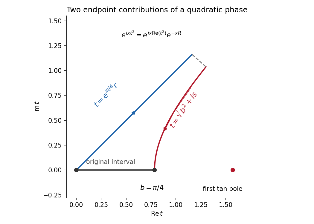
The quadratic phase descends from the stationary endpoint and from the nonstationary upper endpoint
. Details. 
The only nondegenerate stationary point of a phase of the phase is the endpoint zero. Its usual leading stationary phase method term is proportional to the amplitude there, but . Thus the nominal stationary contribution vanishes.
Expand one order further in the local amplitude: . The rescaling then gives a first nonzero stationary contribution of order , with coefficient in the real integral, as in part (i). Meanwhile the upper endpoint is nonstationary and has nonzero amplitude; its integration by parts contribution is , of order .
Consequently the nonstationary endpoint dominates the first nonzero saddle contribution. A stationary phase method formula retaining only the usual leading saddle term would miss the answer. The full stationary phase method, with the vanishing-amplitude correction and the endpoint term, agrees with method of steepest descent. This is quadratic stationary endpoint with quadratically vanishing amplitude.
Treat as independent variables, with . The chain rule givesTherefore the method of multiple scales isThe unspecified term includes the higher correction in . Only the displayed terms through order are needed to determine the leading slow-amplitude system.
At order one, , soAt order ,The operator sends a constant to itself and sends to minus three times themselves. HenceAn additional homogeneous contribution can be absorbed into the definitions of . There is no resonance forcing at this order; the first amplitude evolution therefore occurs on the chosen slower scale .
The order- equation isUsing and , its resonance coefficients aresecular term are removed by setting these to zero:The eigenvalues of this two-by-two system satisfyThey are real with opposite signs for . Generic initial amplitudes then contain an exponentially growing slow-time component. At either leading endpoint the matrix is nonzero nilpotent matrix, so suitable initial amplitudes give linear slow-time growth; higher-order detuning decides the precise corrected boundary. Outside this interval the leading eigenvalues are purely imaginary and the slow amplitudes remain oscillatory.
Substitution into gives the requested leading instability interval“Can become unbounded” permits special initial amplitudes without growth. The calculation identifies the second instability tongue of a weak Mathieu oscillator and its slow amplitudes for the second Mathieu instability tongue; it is not an assertion that every solution grows throughout the closed interval.
Articles by others on the same topic
There are currently no matching articles.