Past exam of the physics A course of the University of Cambridge / 2015 / Paper 2 / Section C

The free electron model replaces the microscopic ionic potential and interacting electronic motion by independent mobile electrons in a uniform neutralizing background, with approximately parabolic dispersion $ϵ={\hslash }^2{k}^2/(2m^{\ast })$. Its quantum version fills states according to Fermi-Dirac statistics and the Pauli exclusion principle. Scattering is represented by a momentum relaxation time $\tau$, rather than derived from the model's ideal free trajectories. This model explains a Fermi energy much larger than room-temperature thermal energy, an electronic heat capacity proportional to temperature at low temperature, and a Drude electrical conductivity. With appropriate scattering assumptions it also yields the Wiedemann-Franz law. It cannot by itself explain band gaps, detailed band anisotropy, strong correlations, or the microscopic temperature dependence of $\tau$.

The inertial term is mass times the rate of change of mean drift velocity. The electric force is $eE$, taking the printed $e$ as the signed electron charge, and $-\gamma ⟨v⟩=-m^{\ast }⟨v⟩/\tau$ describes loss of directed momentum to scattering. electrons retain large microscopic velocities; this damping is of their mean directed motion. In a steady DC field,Both charge factors are negative for electrons, so the conductivity is positive. If $e$ instead denotes a positive charge magnitude, the force and current equations each require a minus sign and give the same result.

For AC response choose physical fields as real parts of phasors proportional to $e^{-i\omega t}$. Substitution givesThusThe real part decreases from ${\sigma }_0$ to zero. The imaginary part starts at zero, reaches ${\sigma }_0/2$ at $\omega \tau =1$, and falls as $1/\omega$. The real part falls as $1/{\omega }^2$ at high frequency. With an $e^{+i\omega t}$ convention, only the sign of the imaginary part changes. Positive $\mathrm{Re}\sigma$ gives positive cycle-averaged dissipation $⟨jE⟩=\mathrm{Re}\sigma |\hat{E}{|}^2/2$.

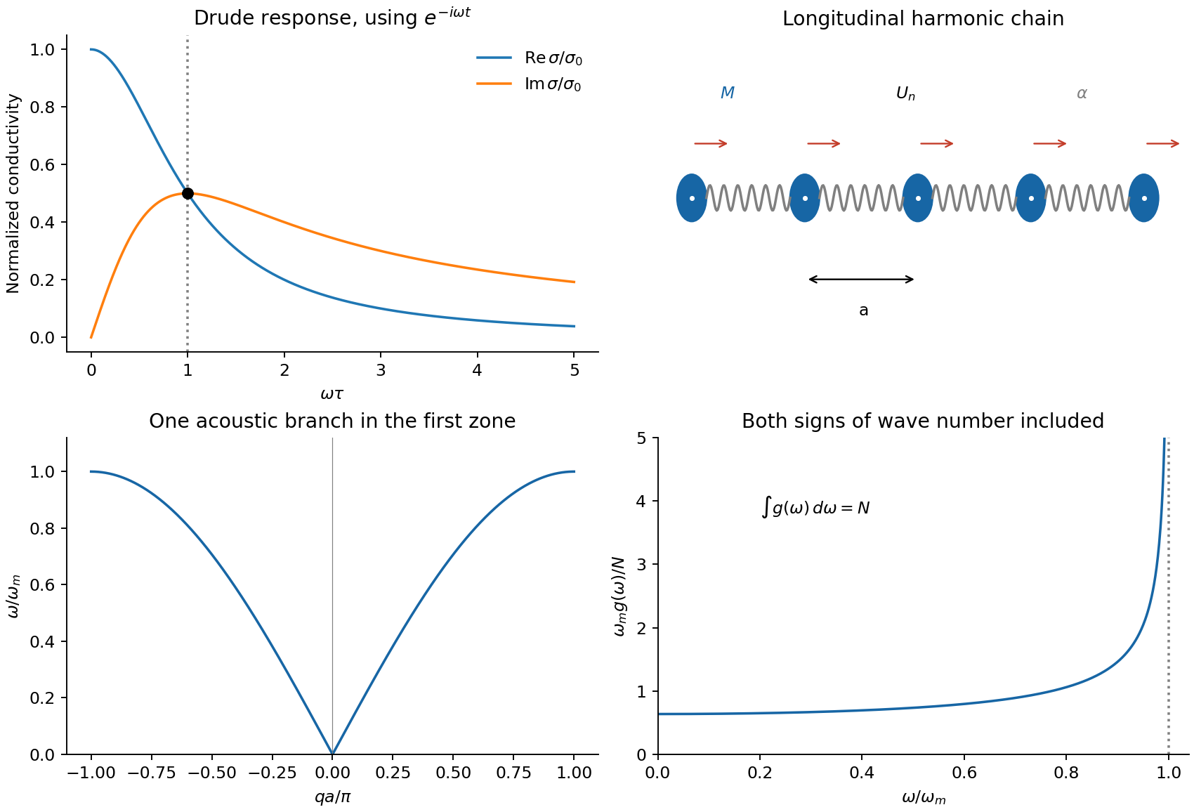
The supplied DC conductivity determines the transport time:Inertia matters when $\omega \tau \sim 1$, giving ${\omega }_c\simeq 4.02\times 10^{13}\mathrm{rad}{\mathrm{s}}^{-1}$, or ${\nu }_c={\omega }_c/(2\pi )\simeq 6.40\times 10^{12}\mathrm{Hz}$. Quoting the former number as hertz would introduce an erroneous factor of $2\pi$.

Write the real displacement as $U_n(t)=\mathrm{Re}[u{e}^{i\omega t-iqna}]$, choosing real positive peak amplitude $u$. Nearest-neighbour harmonic springs store energy in their extension $U_n-U_{n+1}$, each spring counted once. Therefore the instantaneous physical energy isThe printed complex displacement is a calculation device: squaring the complex phasor itself would not produce physical energy. The chain sketch in the accompanying figure shows masses at equilibrium spacing $a$, with longitudinal displacements along the chain.

The two spring forces on site $n$ giveSubstituting the normal-mode phasor and cancelling its nonzero amplitude givesThe long-wavelength limit is acoustic, $\omega \simeq a\sqrt{\alpha /M}|q|$, and the first Brillouin zone ends at $|q|=\pi /a$. The maximum angular frequency is ${\omega }_m=2\sqrt{\alpha /M}$.

Time averaging uses $⟨[\mathrm{Re}(z{e}^{i\omega t}){]}^2⟩=|z{|}^2/2$. ConsequentlyThe dispersion relation makes these two contributions equal, givingThis is equality of time-averaged kinetic and potential energies in a harmonic normal mode; the instantaneous energy partition need not be equal.

Use periodic boundary conditions on length $L=Na$ to count modes: $q_j=2\pi j/L$. The density on the signed $q$ axis is $L/(2\pi )$. Using folded wave-number counting for a monatomic chain combines $q$ and $-q$ at positive magnitude and counts both directions, so the convention used by the requested expression isThis is a large-$N$ continuum density, not a second independent branch. It gives $N$ modes after integrating over that half-zone; endpoint counting changes only finite-size corrections.

For positive $q$, $\omega ={\omega }_m\sin (qa/2)$ andThe density of states of a monatomic harmonic chain vanishes outside the band, is constant to leading order near zero, and has an integrable Van Hove singularity at the upper band edge where group velocity vanishes. Normalization checks the directional counting: