Oceanic magnetic anomalies. Newly formed oceanic crust contains magnetic minerals. As it cools through their magnetic blocking temperatures, it acquires thermoremanent magnetization recording the ambient field polarity. Continuing seafloor spreading carries that record away from the ridge. Geomagnetic reversals therefore generate approximately paired marine magnetic stripes parallel to the ridge, with older crust farther from its axis. A magnetometer measures the superposed field above this magnetized material; subtracting a reference field reveals magnetic anomalies. The anomaly sign and shape depend on magnetization direction, latitude, source depth and geometry, so a positive measured anomaly is not universally identical to normal rock polarity.[ref]
Developing the theory by United States Geological Survey. Sections Magnetic striping and polar reversals, and Seafloor spreading and recycling of oceanic crust
Matching a sequence of stripes to an independently dated reversal chronology gives plate ages and spreading histories. A stripe of width formed over interval implies half-spreading rate under steady symmetric spreading; full separation speed is . Unequal widths on opposite flanks can reflect asymmetric spreading or later deformation. Alteration, remagnetization and overlapping magnetic sources complicate inversion. The sequence correlation is stronger evidence than an isolated stripe or a field-strength peak.
Rayleigh-Bénard convection. Consider a horizontal fluid layer of thickness , hotter below by . The conductive state is motionless with a linear temperature gradient. A rising warm parcel is buoyant, but viscosity resists its motion and thermal diffusion erases its temperature anomaly. In the Boussinesq approximation, density variations are retained in buoyancy while the flow is otherwise incompressible. The competing effects are measured by the Rayleigh number and Prandtl number,For stress-free impermeable, fixed-temperature boundaries, linear stationary disturbances with horizontal wavenumber giveMinimizing gives and the critical Rayleigh number for an isothermal layer, . Two rigid no-slip, fixed-temperature boundaries instead give approximately ; the critical value is not independent of boundary conditions.[ref]
Boundary layer turbulence by Massachusetts Institute of Technology. Chapter 20, §20.4, critical value for two rigid isothermal plates
Above onset, buoyancy can sustain overturning rolls and heat transfer exceeds pure conduction, with Nusselt number . Nonlinear advection eventually limits the disturbance; larger driving can produce time-dependent or turbulent states. The ideal Boussinesq problem does not require hexagonal cells: planform selection depends on boundaries and non-Boussinesq effects. Convection driven by surface tension at a free surface is a distinct mechanism. An adverse temperature gradient supplies driving, but overcoming diffusion and viscosity requires a finite threshold.
Earthquake location. The hypocentre is rupture initiation; its surface projection is the epicentre. Record calibrated arrival times at stations of known coordinates, identify P wave and S wave phases, and predict their travel times through a stated velocity model. Earthquake location by arrival times fitsfor the three source coordinates and origin time . Linearization supplies residual equations . A grid search or iterative weighted least squares inversion can use pick uncertainties, while station geometry controls whether those parameters are well constrained. Four independent arrival constraints are the minimum for four unknowns, not a guarantee of a reliable solution.
In a homogeneous medium, an arrival-time difference between an S wave and a P wave cancels origin time and estimates source-to-station distance,Several distances intersect to locate the event; real layered or three-dimensional Earth structure requires curved-ray travel times. Nearby stations and diverse takeoff angles help resolve depth. Clock errors, phase misidentification, poor azimuthal coverage and incorrect velocities introduce uncertainty or systematic bias. Closely spaced earthquakes can be relocated precisely relative to each other because common-path errors partly cancel, even when their absolute locations remain uncertain. Report a location uncertainty and model assumptions, not merely a best-fit point.
H. F. Reid's earthquake-cycle model. A fault can remain locked while long-term tectonic motion slowly deforms the surrounding rocks. Elastic strain energy and shear stress accumulate. When resistance is overcome, rapid fault slip releases part of that stored energy as seismic waves, frictional heat and other irreversible work. The adjoining rocks partly recover their elastic distortion while retaining a permanent displacement discontinuity across the fault: this is elastic rebound. Surface markers initially crossing the fault become bent during loading and offset after slip.[ref]
Reid's Elastic Rebound Theory by United States Geological Survey. Explanation of gradual strain accumulation, sudden release and the displaced fence; cites Reid's 1910 report, especially pp. 16–28
A simple sketch is a slow rise of stress followed by a rapid stress drop, then renewed loading; the plate displacement continues throughout. Geodetic deformation, observed fault offsets and earthquake stress changes can test the picture. Actual cycles need not repeat with identical slips or times: creep, afterslip, stress transfer and heterogeneous friction complicate the idealization. The release need not remove all pre-existing stress. Elastic rebound explains storage and release; it is not a deterministic earthquake clock.
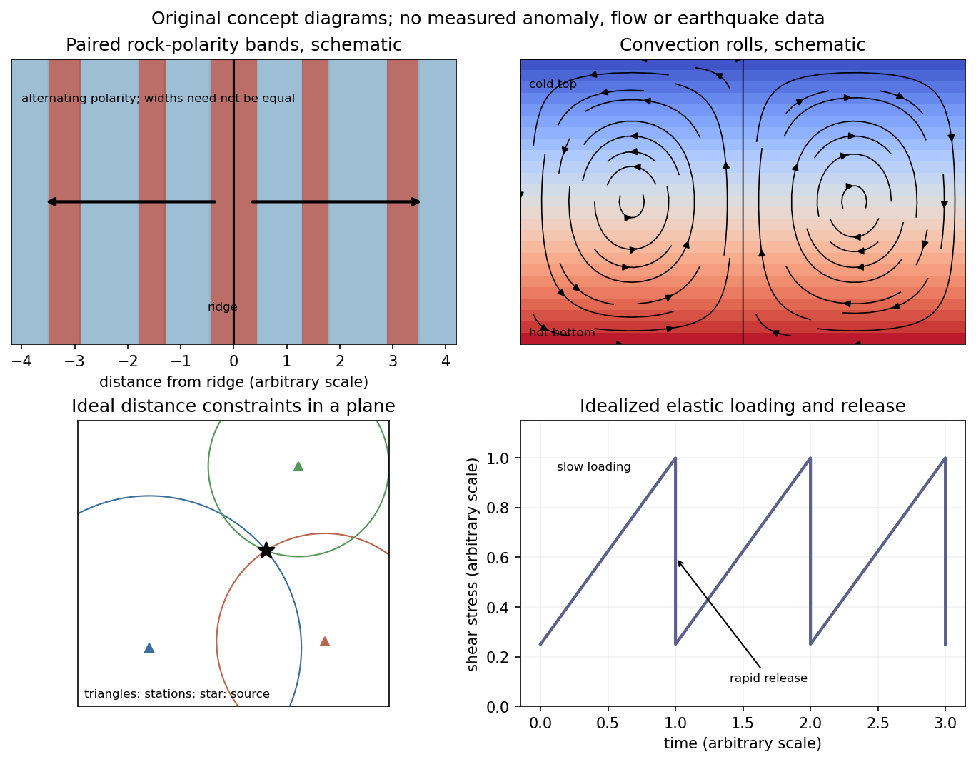
Schematic magnetic stripes, convection rolls, arrival-distance constraints and elastic loading–release cycle; no measured data
. Details. 
Articles by others on the same topic
There are currently no matching articles.