In the oceanic plate cooling model, is temperature, height above the plate base, plate thickness, and age since formation at the spreading axis. With half-spreading rate , a parcel at distance has . The surface and basal temperatures are and respectively. The positive integer labels a sine diffusion mode. For constant thermal diffusivity ,Substituting one sine mode into fixes this normalization; itself is the diffusion timescale before the factor .
Source qualification. The printed transient coefficients have the wrong sign for the intended initially hot plate. Indeed, in the interior,Thus the literal zero-age profile is , where , rather than . It would even approach from inside the upper boundary. The intended hot-ridge cooling solution reverses the transient sign, using . Both versions have the same boundary temperatures and old-age limit. Part (b) gives both surface-flux expressions; the physical ridge-elevation and ridge-push calculations explicitly use the hot initial plate. This sign is present in the original PDF as well as the held transcription.
At the top, . Ocean water provides a cold thermal reservoir relative to mantle temperatures, so a fixed surface temperature is a useful idealization. The model does not resolve near-axis hydrothermal circulation or spatially variable bottom-water temperatures.
At the ridge axis, for in the intended cooling model. Upwelling and magmatic heat supply continually bring hot material into the newly formed plate. The abrupt meeting of this hot interior with the cold upper boundary is an idealized corner discontinuity, resolved diffusively for . The printed series fails this initial condition, as shown in the parent Solution.
At the bottom, . Convecting mantle is treated as maintaining the basal temperature and supplying heat to the plate. This is a prescribed thermal boundary at fixed thickness, not a claim that the real mechanical base is an impermeable material interface.
Far from the ridge, . Transients have decayed and the heat equation reduces to . A finite basal heat supply sustains this gradient. Thermal thickness, seafloor depth and surface heat flux therefore approach finite limits rather than continuing the laws of the half-space cooling model indefinitely.
Take positive heat flux upwards, along increasing , and denote thermal conductivity by . Fourier's law gives . Since , differentiation of the literal printed expression givesIts negative young-age flux is another sign of the unphysical initial profile. For the explicitly corrected hot initial plate, the surface heat flux of a cooling plate is insteadThe old-age limit is . For , replacing the Gaussian sum by its leading integral gives , recovering the half-space cooling model. Neither nor is numerically specified, so the age-dependent flux remains symbolic as requested.
Use the intended hot-ridge state and a linear law of thermal expansion about mantle density at . Let be depth below the old seafloor. Its excess density isand its excess column mass is . Isostasy requires equal pressure at a compensation depth below both columns. Lowering the old seafloor by replaces rock by water, reducing column mass by . Therefore the isostatic ridge elevation in a plate model isHere ; the result is a first-order estimate and neglects sediments, crustal-composition differences and flexural support. If one instead insists on the literal printed zero-age profile, its column is denser than the old plate and the formal relative elevation reverses sign, to this order. That profile cannot describe the elevated hot ridge posited by the question.
Ridge push is a horizontal pressure force integrated with depth, equivalently a difference in gravitational potential energy per horizontal area. It is not the weight of a slab multiplied by the surface slope at one chosen point.
For an explicit compensated-column derivation, let measure depth below the ridge seafloor; the old seafloor is at . Set . The hot column has greater pressure. Its pressure excess over the old column isThe second line follows by integrating upwards from the compensation level. The two expressions agree at because . Integrating this positive pressure excess gives the ridge-push force in a plate model, directed away from the ridge:Consistently retaining only first order in thermal expansion givesIf the topographic term is retained within the same linear-density column model, it adds , giving . This is a useful small correction, not a claim that all other second-order material effects have been included. Both values use the intended hot initial plate, not the inconsistent printed zero-age profile.
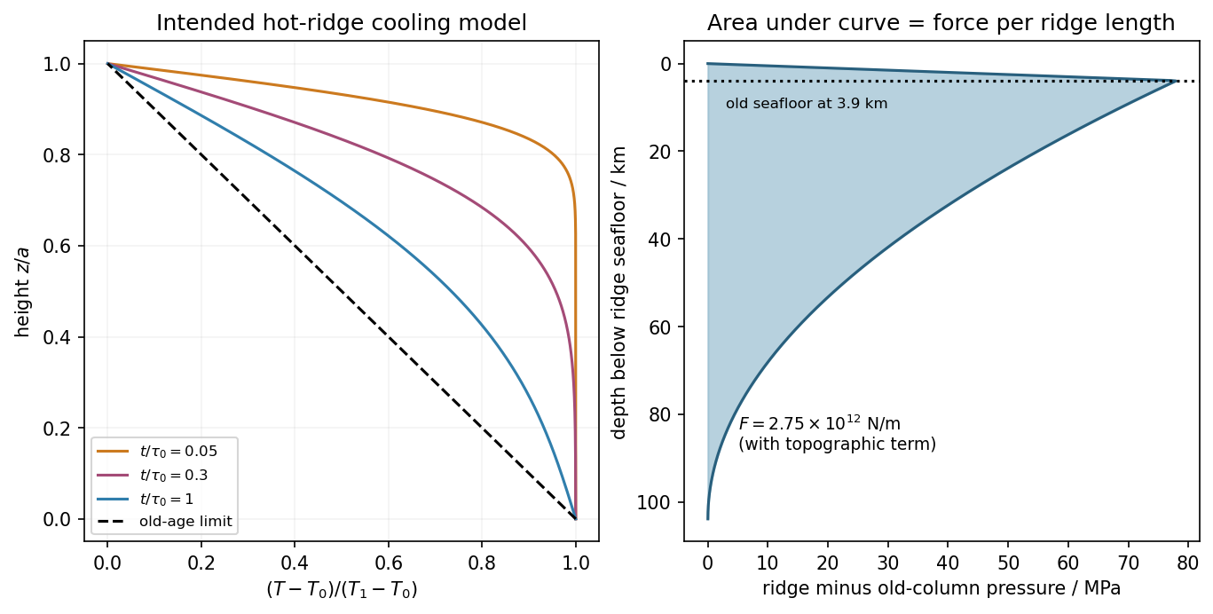
Hot-ridge and old-plate columns, and their compensated pressure difference in the intended cooling model
. Details. The depth-averaged added horizontal compressive stress is . Resolving its traction on a plane dipping at angle gives the fault shear stress from a plate-integrated force,Keeping the previous topographic correction gives about . This is the mean additional shear from ridge push, assuming the force is transmitted through thickness and resolving the nonisotropic stress increment. An isotropic lithostatic pressure adds normal traction but no shear. The force integral alone does not specify the local stress at each point on the fault or establish failure.
Oceanic magnetic anomalies. Newly formed oceanic crust contains magnetic minerals. As it cools through their magnetic blocking temperatures, it acquires thermoremanent magnetization recording the ambient field polarity. Continuing seafloor spreading carries that record away from the ridge. Geomagnetic reversals therefore generate approximately paired marine magnetic stripes parallel to the ridge, with older crust farther from its axis. A magnetometer measures the superposed field above this magnetized material; subtracting a reference field reveals magnetic anomalies. The anomaly sign and shape depend on magnetization direction, latitude, source depth and geometry, so a positive measured anomaly is not universally identical to normal rock polarity.[ref]
Developing the theory by United States Geological Survey. Sections Magnetic striping and polar reversals, and Seafloor spreading and recycling of oceanic crust
Matching a sequence of stripes to an independently dated reversal chronology gives plate ages and spreading histories. A stripe of width formed over interval implies half-spreading rate under steady symmetric spreading; full separation speed is . Unequal widths on opposite flanks can reflect asymmetric spreading or later deformation. Alteration, remagnetization and overlapping magnetic sources complicate inversion. The sequence correlation is stronger evidence than an isolated stripe or a field-strength peak.
Rayleigh-Bénard convection. Consider a horizontal fluid layer of thickness , hotter below by . The conductive state is motionless with a linear temperature gradient. A rising warm parcel is buoyant, but viscosity resists its motion and thermal diffusion erases its temperature anomaly. In the Boussinesq approximation, density variations are retained in buoyancy while the flow is otherwise incompressible. The competing effects are measured by the Rayleigh number and Prandtl number,For stress-free impermeable, fixed-temperature boundaries, linear stationary disturbances with horizontal wavenumber giveMinimizing gives and the critical Rayleigh number for an isothermal layer, . Two rigid no-slip, fixed-temperature boundaries instead give approximately ; the critical value is not independent of boundary conditions.[ref]
Boundary layer turbulence by Massachusetts Institute of Technology. Chapter 20, §20.4, critical value for two rigid isothermal plates
Above onset, buoyancy can sustain overturning rolls and heat transfer exceeds pure conduction, with Nusselt number . Nonlinear advection eventually limits the disturbance; larger driving can produce time-dependent or turbulent states. The ideal Boussinesq problem does not require hexagonal cells: planform selection depends on boundaries and non-Boussinesq effects. Convection driven by surface tension at a free surface is a distinct mechanism. An adverse temperature gradient supplies driving, but overcoming diffusion and viscosity requires a finite threshold.
Earthquake location. The hypocentre is rupture initiation; its surface projection is the epicentre. Record calibrated arrival times at stations of known coordinates, identify P wave and S wave phases, and predict their travel times through a stated velocity model. Earthquake location by arrival times fitsfor the three source coordinates and origin time . Linearization supplies residual equations . A grid search or iterative weighted least squares inversion can use pick uncertainties, while station geometry controls whether those parameters are well constrained. Four independent arrival constraints are the minimum for four unknowns, not a guarantee of a reliable solution.
In a homogeneous medium, an arrival-time difference between an S wave and a P wave cancels origin time and estimates source-to-station distance,Several distances intersect to locate the event; real layered or three-dimensional Earth structure requires curved-ray travel times. Nearby stations and diverse takeoff angles help resolve depth. Clock errors, phase misidentification, poor azimuthal coverage and incorrect velocities introduce uncertainty or systematic bias. Closely spaced earthquakes can be relocated precisely relative to each other because common-path errors partly cancel, even when their absolute locations remain uncertain. Report a location uncertainty and model assumptions, not merely a best-fit point.
H. F. Reid's earthquake-cycle model. A fault can remain locked while long-term tectonic motion slowly deforms the surrounding rocks. Elastic strain energy and shear stress accumulate. When resistance is overcome, rapid fault slip releases part of that stored energy as seismic waves, frictional heat and other irreversible work. The adjoining rocks partly recover their elastic distortion while retaining a permanent displacement discontinuity across the fault: this is elastic rebound. Surface markers initially crossing the fault become bent during loading and offset after slip.[ref]
Reid's Elastic Rebound Theory by United States Geological Survey. Explanation of gradual strain accumulation, sudden release and the displaced fence; cites Reid's 1910 report, especially pp. 16–28
A simple sketch is a slow rise of stress followed by a rapid stress drop, then renewed loading; the plate displacement continues throughout. Geodetic deformation, observed fault offsets and earthquake stress changes can test the picture. Actual cycles need not repeat with identical slips or times: creep, afterslip, stress transfer and heterogeneous friction complicate the idealization. The release need not remove all pre-existing stress. Elastic rebound explains storage and release; it is not a deterministic earthquake clock.
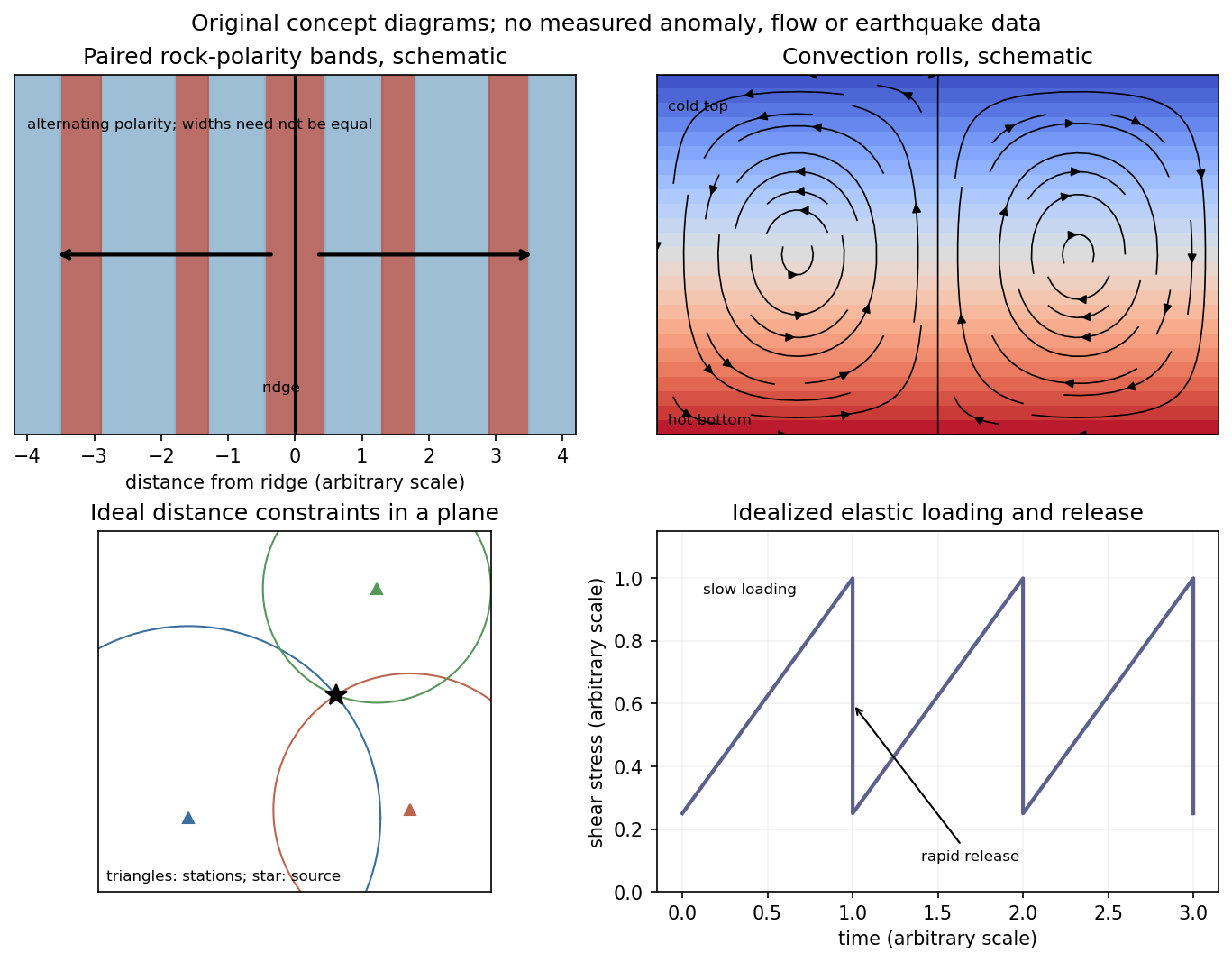
Schematic magnetic stripes, convection rolls, arrival-distance constraints and elastic loading–release cycle; no measured data
. Details. For group velocity from a period-dependent phase velocity, start with rather than equating group velocity to phase velocity. Differentiating,For the stated inverse-frequency term, , soThe inequality assumes positive frequency and physical positive phase velocity, with . The symbol here has units of acceleration and is unrelated to the plate thickness in Question 1.
Write the oscillation period as , so locally . The first overtone is the lowest curve above the fundamental, not the fundamental mode itself. Near , Figure 1 gives approximately . Representative nearby readings are about at and at . ThusThe local group-velocity estimate isThese are graphical estimates, roughly and , rather than high-precision fitted constants. The nearby straight-line approximation need not describe that mode over the whole plotted period range. No source curve is reproduced here.
The phase velocity in Figure 1 is measured along the Earth's surface. Spherical geometry makes the local horizontal phase speed at radius equal to . In the ray approximation, squared radial shear wavenumber isThe spherical surface-wave evanescence threshold immediately below the discontinuity is thereforeEquality is the grazing limit. Using directly would omit the requested spherical correction. Immediately above the discontinuity the corresponding boundary is . Hence the interval specifically describes propagation just above the jump and evanescence just below it. Slower modes can already be evanescent above .
Intersecting the plotted branches with gives the following approximate upper periods. Below each upper period, that branch is evanescent immediately beneath the discontinuity:
- fundamental mode: throughout the displayed – range;
- first and second overtones: approximately and ;
- successive higher curves: approximately , , , , and .
For these overtones the displayed ranges thus start near and end at their respective crossings. Any still higher curve already above the threshold at the lower plotted period has no evanescent interval within the displayed range. Readings of the closely spaced higher curves are only accurate to about a second, and the plot does not establish their continuation to unshown periods. Nor does the local inequality prove that a mode remains evanescent at every greater depth in an unspecified Earth model.
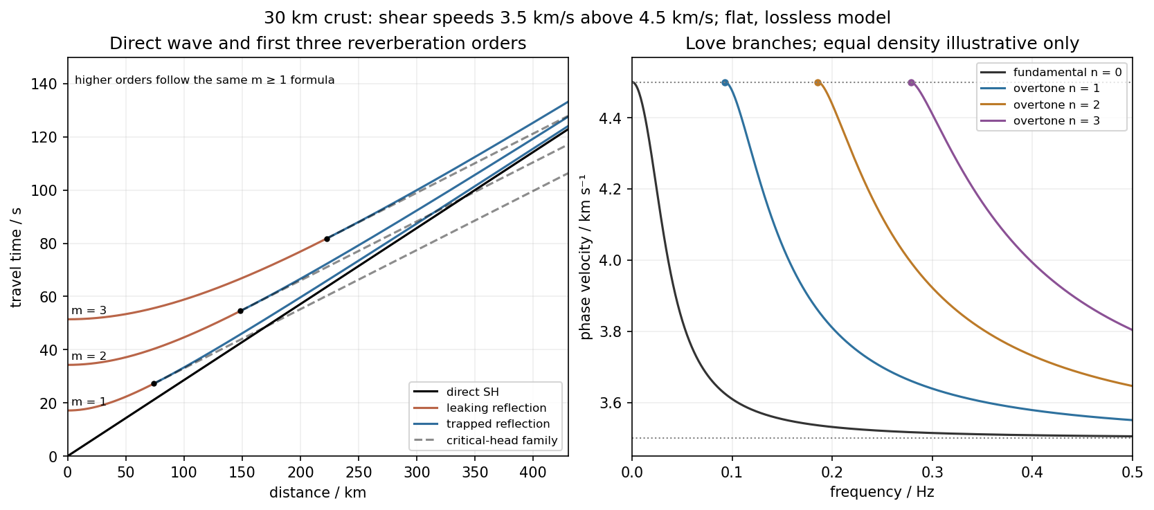
Use the flat two-layer model, with thickness , crustal shear speed and mantle speed . For SH-wave travel times in a crustal waveguide, unfolding each reflected path gives all reflection orders at once:with in kilometres and times in seconds. The direct wave begins at the origin; reflected orders have intercepts and approach the direct-wave slope at large distance.
The critical angle, measured from the vertical, is . Associated critical refraction and its multiples giveEach head-wave line is tangent to its reflection curve at the critical distance. In particular the primary head wave exists before it becomes the first arrival; it overtakes the direct wave only around .
The slope of a reflected travel-time curve is . For , , so the mantle supports outgoing shear radiation and successive reverberations leak energy. For , : the mantle field is evanescent and ideal interface reflection is total. These leaking and trapped SH-wave reverberations explain the annotations in the original travel-time drawing below. A reflected ray is not itself a separate Love mode: constructive interference of the trapped contributions, including reflection phase, selects the normal modes.
For a horizontally propagating mode with , define vertical wavenumbersThe free upper surface and welded interface impose the Love-wave dispersion conditionwhere are shear moduli. Each phase-velocity branch falls towards with increasing frequency. Higher branches join at their low-frequency cutoffs. At cutoff , soThus the first three overtones have maximum periods about , and . The fundamental mode has and no positive-frequency cutoff in this flat layer-over-half-space model: it approaches as , with ever-deeper penetration. The phase-velocity sketch uses an explicitly illustrative equal-density choice, because the question gives speeds but no density or rigidity ratio. That missing ratio changes detailed branch curvature, not the cutoff values or the requested branch topology.
For the actual finite spherical Earth, the very-long-period continuation must instead be described by discrete toroidal normal modes, not a flat infinite waveguide at arbitrary wavelength. The flat-model answer therefore does not assert a continuum of arbitrarily low-frequency global nonrigid oscillations. A global lowest oscillation frequency cannot be computed from the supplied crust-and-half-space data alone.[ref]
Essentials of Geophysics: Seismology by R. D. van der Hilst. §4.18, Love-wave trapping; §4.23, finite spherical Earth and discrete normal modes, especially printed pp. 184–187


Articles by others on the same topic
There are currently no matching articles.