Optical depth increases downward because dτ=−kρdz. Along an upward ray the beam loses irradiance by absorption, as in Beer-Lambert attenuation, and gains it from local thermal emission. Kirchhoff's law equates emissivity and absorptivity in local thermodynamic equilibrium, giving source term πB. Thus −dI/dτ=−I+πB, equivalently the given equation. The factor π converts isotropic radiance into hemispheric irradiance in the stipulated diffuse approximation. The following two limits hold for the same downward optical-depth coordinate.
With negligible atmospheric emission, dI/dτ=I. If the warm surface is at τs, I(τ)=Ise−(τs−τ). Irradiance decreases as the beam travels upward to smaller τ, and I(0)=Ise−τs. The positive derivative with respect to downward optical depth is consistent with attenuation, not amplification along propagation.
For an infinitely deep isothermal atmosphere the bounded solution is I(τ)=πB. A more general formal solution contains Ceτ, excluded by the bounded deep boundary condition. Emission exactly replenishes absorption, so the emergent spectrum is blackbody in this idealized wavelength-by-wavelength thermal model.
Multiplying I′−I=−πB by e−τ gives (Ie−τ)′=−πBe−τ. Integrating to depth T yields I(0)=I(T)e−T+π∫0TB(t)e−tdt. If the first term vanishes as T→∞,Each layer emits in proportion to Bdτ and is attenuated by its overlying optical depth. The normalized exponential weighting emphasizes optical depths of order unity, while retaining contributions from a range of heights.
I0=π∫0∞B(τ)e−τdτ.
Hydrostatic balance and the ideal gas law give dp/dz=−pg/(RaT), hence approximately p=p0e−z/H with H=RaT/g for weak temperature variation. For well-mixed absorber abundance, ρabs∝p/T, while pressure broadening gives k∝p. Thus kρabs∝e−2z/H and its integral above height z has the same scale. ThereforeThe factor two depends on both pressure dependence of absorption and constant mixing ratio; it is not the ordinary density scale height.
τ(z)∝e−z/Hτ,Hτ=RaT/(2g).
Let τt be the tropopause optical depth and linearize B with positive derivative BT. In the troposphere T=Tt+ΓHτlog(τ/τt), so the requested schematic isIt is constant in the isothermal stratosphere and rises linearly with logτ below it. At unchanged temperatures and a multiplicative abundance change a, optical depth at each height changes to aτ, hence Ba(τ)=Bold(τ/a). Doubling moves the tropopause kink to 2τt and gives colder emission temperatures at a fixed optical depth; halving does the opposite.
B(τ)={Bt,Bt+BTΓHτlog(τ/τt),τ≤τt,τ>τt.
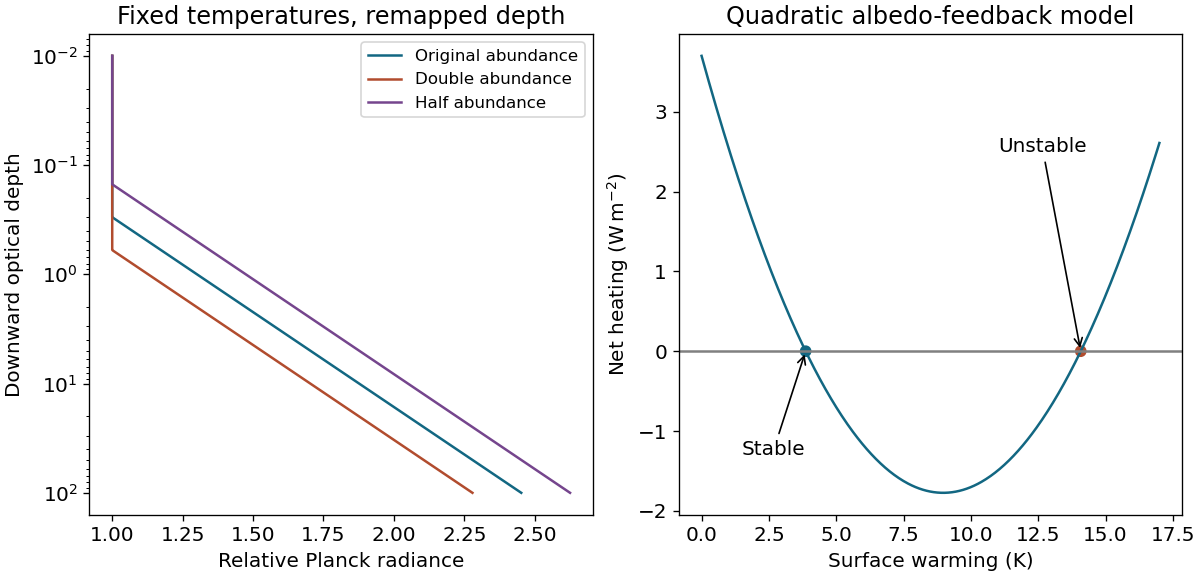
Optical-depth remapping of atmospheric emission and stable versus unstable climate-feedback equilibria
. Details. 
For dry ascent, cpdT=Vdp and hydrostatic pressure change is dp/dz=−ρg=−g/V, so Γd=−dT/dz=g/cp. During condensation dq<0, and −Ldq>0 offsets expansion cooling, making the saturated ascent less steep.
For a saturated parcel with q=qs(T,p), use dq=qTdT+qpdp to obtainWith dilute vapor, qp≃−qs/p and qT≃Lqs/(RvT2), this becomes Γd[1+Lqs/(RaT)]/[1+L2qs/(cpRvT2)]. In terrestrial conditions the denominator's latent-heating correction dominates. Warming increases saturation humidity strongly, so latent heat increasingly compensates expansion cooling and the moist lapse rate falls. This is a statement about saturated convective adjustment, not every instantaneous environmental temperature profile.
Γm=cp+LqTg(1−Lqp/V).
Effective emission temperature satisfies σTe4=S0(1−α)/4: absorbed sunlight over the planetary disc balances radiation over the whole sphere. Thus Te=[S0(1−α)/(4σ)]1/4. Taking S0=1360 W m−2 gives about 254.5 K. If only a uniform atmospheric/surface temperature shift is allowed, the blackbody response coefficient is λP=4σTe3≃3.74 W m−2 K−1. HenceThe surface and troposphere shift together under this fixed-profile approximation; their absolute temperatures need not equal Te. A more detailed spectral Planck feedback requires additional information not supplied by the simple model.
ΔT≃3.7/λP≃0.99 K.
At a fixed surface warming, a smaller lapse rate makes the upper troposphere warmer than in an unchanged-lapse profile. Its emission to space therefore increases, giving a negative feedback. Water vapor has the opposite effect under the given coefficients. The net restoring coefficient is λP−2+0.5≃2.24 W m−2 K−1, so ΔT≃1.65 K. This calculation uses the same S0 and linearized Planck model as the preceding part.
Albedo reduction increases absorbed short-wave flux by S0(a1T+a2T2)/4. Define A=λP−1.5−S0a1/4 and B=S0a2/4. The perturbation energy balance is N(T)=F−AT+BT2, where F=3.7 W m−2 for doubling. With the preceding constants, A≃1.220 W m−2 K−1 and B=0.068 W m−2 K−2. The two roots areStability follows from N′(T)=−A+2BT<0 at the lower root. They merge at T=A/(2B)≃8.97 K and Fmax=A2/(4B)≃5.47 W m−2; at equality the equilibrium is marginal, not linearly stable.
Tstable≃3.86 K,Tunstable≃14.1 K.
Assuming the usual logarithmic forcing extension F=3.7log(C/280)/log2 gives a stable branch only for C<Ccrit≃7.8×10² ppm. This “maximum” is the supremum of stable concentrations in the stated quadratic, linearized model. It is not a physical prediction of a real-world runaway threshold; extrapolating its feedback laws far beyond their small-change regime is an additional assumption.
The second box represents a reservoir exchanging carbon with the atmosphere, with equal capacity in the chosen concentration units. For a unit atmospheric pulse, C(0+)=1, C1(0+)=0 and no subsequent emissions, total C+C1=1 is conserved while d(C−C1)/dt=−2k(C−C1). ThusThe atmospheric burden falls from one to one half with time constant (2k)−1, not k−1. The model has a permanent airborne fraction because neither box contains an external sink. The carbon-response panel of the original figure in S12 shows this explicitly.
C(t)=21(1+e−2kt),C1(t)=21(1−e−2kt).
For a small additional carbon mass, logarithmic forcing has derivative inversely proportional to the background atmospheric carbon inventory. With other conversion factors fixed, b0 therefore decreases as background concentration rises. Solve the temperature equation using an integrating factor and the pulse burden:At b1=2k the second term is its continuous limit te−b1t. For 0<k≪b1, temperature initially rises over b1−1 toward roughly b0/b1, then relaxes over (2k)−1 toward half that value. This produces an overshoot, rather than permanent growth. The two numerical limits requested separately below also follow directly from the differential equation.
T(t)=2b0[b11−e−b1t+b1−2ke−2kt−e−b1t].
Temperature is continuous through an instantaneous carbon injection. With T(0)=0 and C(0+)=1, T˙(0+)=b0. Its initial slope is finite; the emission pulse makes the carbon burden jump but does not give this first-order thermal model an instantaneous temperature jump.
At late times C→1/2 and thermal equilibration requires b0C−b1T=0. Hence T(∞)=b0/(2b1). Both t≫k−1 and t≫b1−1 ensure that the exchange and thermal transients have decayed.
For constant marginal annual damage D′ and positive discount rate r, use the Laplace transform of the preceding equations:The approximation uses r≪b1 but does not require choosing an order between r and k. At zero discount rate the integral diverges in this model because the pulse leaves permanent positive warming and damages remain constant per degree.
C(r)=r(r+2k)r+k,SC−CO2=r(r+2k)(r+b1)D′b0(r+k)≃2b1D′b0(r1+r+2k1).
If economic activity is adapted to the old climate, additional warming generally pushes temperatures, water availability and extremes further from that adapted range. With convex aggregate damages, marginal annual damage per degree D′ therefore tends to rise as the world warms. This is an argued expectation under the stated adaptation baseline, not a theorem: adaptation, wealth changes, regional benefits and thresholds alter both the level and curvature of damages. A constant D′ in the preceding integration is a simplifying local approximation, and may understate later losses when convexity dominates.
Ancestors (9)
- 2017
- Past exam of the short options paper shared by Prelims and Parts A and B of the physics course of the University of Oxford
- Short options paper shared by Prelims and Parts A and B of the physics course of the University of Oxford
- Physics course of the University of Oxford
- Undergraduate course of the University of Oxford
- Course of the University of Oxford
- University of Oxford
- List of universities
- Home
Discussion (0)
New discussionThere are no discussions about this article yet.
Articles by others on the same topic (0)
There are currently no matching articles.