Past exam of the short options paper shared by Prelims and Parts A and B of the physics course of the University of Oxford / 2017 (A14119/A15348/A14140/A15349/A15351/A15350/A15352)

Source paper: www.whatdotheyknow.com/request/oxford_physics_past_papers_2/response/2340696/attach/5/Physics%20Papers%202016.pdf?cookie_passthrough=1. The cover dates the whole booklet to Trinity Term 2017, 13 June; the 2016 bundle filename does not control the year. Unlettered marked requests are numbered in their source order; explicitly lettered requests retain their letters. Section S18 has publicly advertised answer notes, which cover only that option rather than this twelve-option booklet.

Complex differentiability gives $u_x=v_y$, $u_y=-v_x$. Differentiating once more, for continuously differentiable first derivatives with the needed second derivatives, yields $u_{xx}+u_{yy}=v_{yx}-v_{xy}=0$ and $v_{xx}+v_{yy}=-u_{yx}+u_{xy}=0$. Thus both components satisfy Laplace's equation. The result is local on the domain of holomorphy; it makes no assertion across a branch cut.

Choose a continuous argument $\theta$ on a simply connected domain avoiding zero, and put $r=\sqrt{x^2+y^2}$. With $u=x\log r-y\theta$, direct differentiation givesHere ${\theta }_x=-y/r^2$, ${\theta }_y=x/r^2$; these identities specify the branch needed in the written arctangent. Integrating the Cauchy-Riemann equations givesThe literal principal $\arctan (y/x)$ works only separately on suitable half-planes. It cannot stand for a single continuous argument across the imaginary axis.

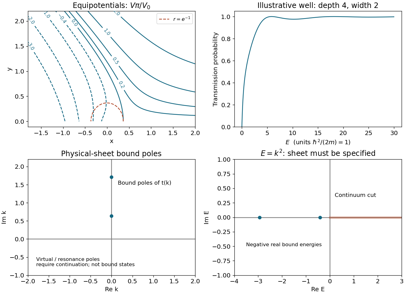
For the upper half-plane use $0<\theta <\pi$, and interpret the source's arctangent as this argument. Then $V=(V_0/\pi )\mathrm{Im}(z\mathrm{Log}z)$ is harmonic, so $\mathbf{E}=-\nabla V$ has zero curl and divergence where there is no charge. On the positive boundary $\theta \to 0$ and $y\log r\to 0$; on the negative boundary $\theta \to \pi$. Hence the two boundary values are respectively zero and $V_{0}x$.

Branch qualification: the principal real arctangent alone gives zero on both sides of $y=0$, contradicting the stated negative-axis boundary condition, for example at $x=-1$. The continuous upper-half-plane argument repairs this notation; it is not an optional additive constant.

Along a level curve, $V_{x}dx+V_{y}dy=0$, with $V_x=V_0\theta /\pi$ and $V_y=V_0(1+\log r)/\pi$. ThereforeIn the intended upper half-plane $0<\theta <\pi$, the slope is positive for $0<r<e^{-1}$, vertical at $r=e^{-1}$, and negative for $r>e^{-1}$. At the positive real boundary $\theta =0$ the slope is zero except at the stationary point $(e^{-1},0)$, where both derivatives vanish and the quotient is indeterminate. More generally, outside the chosen half-plane its sign is the sign of $-\theta (1+\log r)$, with the argument branch held fixed. A convenient parametric description of the curves to sketch is $V\pi /V_0=r(\sin \theta \log r+\theta \cos \theta )$.

A branch point obstructs a single-valued analytic continuation around a closed circuit. Continuing $\log z=\log |z|+i\theta$ once around zero increases its value by $2\pi i$. A branch cut removes a curve joining branch points or extending to infinity so that a continuous argument can be chosen on the remainder. Zero and infinity are logarithmic branch points; the positive-axis cut used here selects $0<\arg z<2\pi$. The cut is a choice of representation, not a line of poles of the multivalued logarithm.

The large circle contributes $O((\log R{)}^n/R)$ and the small circle contributes $O(ϵ|\log ϵ{|}^n)$, so both disappear. The enclosed simple poles are $i$ and $-i$, with logarithms $i\pi /2$ and $3i\pi /2$. Their residues are $(i\pi /2{)}^n/(2i)$ and $-(3i\pi /2{)}^n/(2i)$. The positive orientation of the keyhole therefore givesThe upper bank runs outward and the lower bank inward. Their logarithms differ by $2\pi i$; keeping that orientation is essential for the sign.

Taking the difference of the two bank integrals at $n=2$ givesThe $I_j$ are real and convergent. Comparing real and imaginary parts proves $\boxed{I_0=\pi /2,I_1=0}$. Independently, $x\mapsto 1/x$ changes the sign of each odd logarithmic moment and preserves the measure, so every odd $I_j$ vanishes.

At $n=3$ the bank difference is $-6\pi i{I}_2+12{\pi }^2{I}_1+8{\pi }^{3}i{I}_0$, while the residue result is $13i{\pi }^4/4$. Substitution of $I_0,I_1$ yields $I_2={\pi }^3/8$.

At $n=5$, the odd moments vanish and the remaining relation isThusAs an independent generating-function check, $F(s)={\int }_0^{\infty }{x}^s/(1+x^2)dx=\pi /[2\cos (\pi s/2)]$ for $|\mathrm{Re}s|<1$. Differentiating twice and four times at zero gives the same moments.

For a meromorphic function with no poles on a positively oriented closed contour, the contour integral equals $2\pi i$ times the sum of enclosed residues, weighted by winding number for a general contour. At a simple pole $a$, the residue is ${\lim }_{z\to a}(z-a)f(z)$. Analyticity on the contour and the absence of other interior singularities are necessary hypotheses.

Put $z=e^{i\theta }$, so $d\theta =dz/(iz)$, $\cos \theta =(z+z^{-1})/2$ and $\sin \theta =(z-z^{-1})/(2i)$. Rational expressions in these trigonometric functions become rational contour integrands on the unit circle. The method is especially useful when the resulting denominator has a small number of identifiable poles. A pole on the integration circle requires a separately specified principal value or indentation; the residue theorem does not automatically assign an ordinary integral there.

First remove the removable singularities introduced by tangent and secant: the integrand is $\cos \theta /(3+\cos \theta +2\sin \theta )$. The denominator stays positive since $3>\sqrt{5}$. With $z=e^{i\theta }$ the contour integrand isIts interior poles are zero and $r=-1/(1-2i)$; the other quadratic root is $-5/(1-2i)$ and lies outside. The residues are $1/[i(1+2i)]$ and $(r^2+1)/(4ir)$, whose sum is $i/10$. ConsequentlyAssigning arbitrary finite values at the isolated removable points does not change the integral.

Split the sine into exponentials. The $e^{iz}$ term closes in the upper half-plane and picks up the pole $ia$, giving $2\pi i{e}^{-a}$; the $e^{-iz}$ term closes clockwise below and encloses no pole. Jordan's lemma applies to these separate contours. HenceTo pass to $a\downarrow 0$ without an invalid dominated-convergence argument on an infinite interval, pair positive and negative $x$ first: the imaginary part is odd and the real part is $2{\int }_0^{\infty }x\sin x/(x^2+a^2)dx$. On a bounded interval the limit is harmless, while integration by parts bounds the oscillatory tail uniformly for $0<a\le 1$. This gives the convergent improper Dirichlet integral $\boxed{{\int }_{-\infty }^{\infty }\sin x/xdx=\pi }$.

For two isolated point masses in a Newtonian bound orbit, $\boxed{P^2=4{\pi }^2{a}^3/[G(M_s+M_p)]}$, where $a$ is the relative orbit's semimajor axis. For a negligible planet mass, using years, astronomical units and solar masses gives $(P/\mathrm{yr}{)}^2=(a/\mathrm{AU}{)}^3/(M_s/M_{\odot })$. The mass in the denominator is the total gravitating mass, not the planet's mass alone.

Circular edge-on motion gives $V_s=2\pi a_s/P$ and center-of-mass balance gives $a_s=a{M}_p/(M_s+M_p)$. Eliminate $a$ using the preceding period relation:Thus $\boxed{M_p^3\simeq P{V}_s^3{M}_s^2/(2\pi G)}$ when $M_p\ll M_s$. For a non-edge-on orbit the measured velocity instead determines $M_p\sin i$ to this accuracy; neglecting eccentricity is also part of the stipulated model.

A luminosity does not determine a stellar mass without a mass-luminosity calibration. Using the usual approximate main-sequence law $L/L_{\odot }=(M_s/M_{\odot }{)}^{\alpha }$ gives $M_s=3^{1/\alpha }{M}_{\odot }$. With $\alpha =3.5$, the numerical results areThe angular radius follows directly from $a(\mathrm{AU})/d(\mathrm{pc})$. Taking $\alpha =4$ changes these estimates by only a few percent, but the calibration must be stated. Hubble's 2.4 m aperture has visible-light diffraction scale $1.22\lambda /D\simeq 0.05$ arcsec at 500 nm, hundreds of times larger. The separation is therefore unresolved even before the severe star/planet contrast is considered.

The effective temperature is defined by $\boxed{L=4\pi R_{\ast }^2\sigma T_{\mathrm{eff}}^4}$, with bolometric luminosity $L$, photospheric radius $R_{\ast }$ and Stefan-Boltzmann constant $\sigma$. It is the blackbody temperature giving the same total surface flux, not a claim that each spectral line forms at that temperature.

The parallax gives $d=20$ pc and the distance modulus gives $M_{\mathrm{bol}}=-0.641-5{\log }_{10}2=-2.146$. Therefore $L/L_{\odot }=10^{(4.72-M_{\mathrm{bol}})/2.5}\simeq 558$. Taking $T_{\odot }\simeq 5772$ K,This is a cool luminous giant, in the red-giant region of the Hertzsprung-Russell diagram. On the usual first-ascent interpretation, luminosity comes predominantly from hydrogen shell burning around an inert helium core, with gravitational adjustment also contributing. The two measured quantities alone do not uniquely determine evolutionary history: a later giant phase can overlap this region, so they do not prove the precise core-burning state.

A continuum peak gives a color temperature through Wien's law, provided the continuum is approximately Planckian and extinction is corrected. Broad-band colors or a fitted spectral energy distribution compare flux ratios with model atmospheres; they require a reddening estimate, abundance and gravity assumptions, and calibrated passbands. Spectroscopic line ratios or excitation/ionization balances provide another thermometer, requiring atomic data and a suitable atmosphere model, often local thermodynamic equilibrium.

For this cool giant, line blanketing and molecular absorption substantially distort a simple continuum peak, so Wien's law is the least reliable of these approximations. A detailed spectroscopic analysis, checked against a multi-band atmosphere fit, would generally be the strongest of the three if good data and model parameters are available. There is no unconditional accuracy ranking without measurement errors and model systematics; an accurately measured angular diameter plus bolometric flux would offer a more direct effective-temperature determination, if obtainable.

At a fixed cosmological time, homogeneous expansion has $\mathbf{v}=H(t)\mathbf{r}$. A comoving galaxy has $\mathbf{r}=R(t)\mathbf{x}$ with constant $\mathbf{x}$, hence $\mathbf{v}=\dot{R}\mathbf{x}=(\dot{R}/R)\mathbf{r}$. Thus $\boxed{H=\dot{R}/R}$. Peculiar velocities must be removed before applying this ideal relation to individual galaxies.

Set the spatial-curvature constant to zero in the stipulated matter-only Friedmann equation to get ${\rho }_c=3H^2/(8\pi G)$. Conservation of pressureless matter with $R(t_0)=1$ gives $\rho ={\rho }_0/R^3$, and thereforeChoosing the Big Bang as $t=0$ yields $R=(t/t_0{)}^{2/3}$ and $H=2/(3t)$. Consequently $\boxed{t_0=2/(3H_0)\simeq 9.3\mathrm{Gyr}}$ for the supplied $H_0$. This is the age of the flat pressureless model without a cosmological constant, not a determination in the current multi-component cosmological model.

The matter rest-energy density is ${\rho }_m{c}^2\simeq 2.25\times 10^{-10}$ J m${}^{-3}$, whereas the given photon density is $8.01\times 10^{-14}$ J m${}^{-3}$. Their present ratio is about $2.8\times 10^3$. Matter scales as $(1+z{)}^3$ and freely redshifting radiation as $(1+z{)}^4$, soThis compares matter specifically with the supplied CMB photons. Adding relativistic neutrinos changes the total radiation equality redshift; it is not included in these data.

The Bohr model assumes Coulomb attraction and classical circular motion between transitions; selected stationary orbits do not radiate; their angular momentum is $mvr=n\hslash$; and a transition exchanges a photon of energy $h\nu =E_i-E_f$. The first two dynamical equations giveHere $n=1,2,\dots$, $m$ is the electron mass under the fixed-proton approximation, $e$ its charge magnitude, and ${ϵ}_0$ the vacuum permittivity. The stationary-orbit postulate deliberately suspends the classical radiation prediction; this is a historical model, not a consistent deduction from classical electrodynamics.

Substitute the quantized radius in $mvr=n\hslash$ to get $v_n=e^2/(4\pi {ϵ}_0\hslash n)$. Coulomb potential energy is $-e^2/(4\pi {ϵ}_0{r}_n)$ and the stipulated virial relation makes the total one half of this value. HenceThe negative sign means a bound state relative to a separated stationary proton and electron.

The emitted photon has energy $E_3-E_2=\mathrm{Ry}(1/4-1/9)=5\mathrm{Ry}/36$. ThereforeThis is the Balmer-alpha transition in this approximation. Absorption in the reverse direction has the same photon energy; fine structure and radiative corrections are beyond the model.

Separate center-of-mass motion and replace $m$ by the reduced mass $\mu =mM/(m+M)$ in the relative-coordinate formulas. Then $r_n$ is the proton-electron separation, energy levels and the Rydberg constant scale by $\mu /m$, and transition wavelengths increase by $m/\mu$. The electron's own orbital radius about the center of mass is $M{r}_n/(M+m)$; the proton radius is $m{r}_n/(M+m)$. The relative speed retains $\alpha c/n$, while the electron's individual speed acquires $M/(M+m)$. Replacing the mass in the radius alone but leaving energies unchanged would be inconsistent.

For a stationary nonrelativistic state, $\boxed{[-{\hslash }^2{\nabla }^2/(2m)+V(\mathbf{r})]\psi =E\psi }$. The wavefunction $\psi$ is a probability amplitude, $m$ the particle mass and $E$ its energy eigenvalue; the potential energy $V$ is measured in the same energy units. In one dimension the Laplacian becomes $d^2/d{x}^2$.

Inside the well, ${\psi }^{\prime \prime }+k^2\psi =0$. Vanishing at zero removes the cosine term; vanishing at $L$ requires $k_{n}L=n\pi$. The nonzero states have positive integer $n$ because $n=0$ gives the zero function and negative $n$ only repeats a state up to sign. Normalization follows from ${\int }_0^L{\sin }^2(n\pi x/L)dx=L/2$. ThusThe wavefunction vanishes outside the infinite barriers, so there is no additional contribution to its norm.

A sudden wall displacement leaves the initial wavefunction unchanged: it is $\sqrt{2/L}\sin (\pi x/L)$ on $[0,L]$ and zero on $(L,2L]$. It is not an eigenfunction of the new Hamiltonian, so there is no single certain new energy. Its energy expectation immediately afterward remains $E_1^{\mathrm{old}}$, as seen from ${\hslash }^2\int |{\psi }^{\prime }{|}^2/(2m)$; the measurement outcomes are $E_n^{\mathrm{new}}=n^2{E}_1^{\mathrm{old}}/4$.

The new ground state is $L^{-1/2}\sin (\pi x/(2L))$. Its overlap is $4\sqrt{2}/(3\pi )$, soThe discontinuity of the derivative at the former wall does not invalidate the finite quadratic-form expectation, although it matters when applying the differential Hamiltonian pointwise. Adiabatic expansion would instead keep the state in the ground level and reduce its energy by four.

For a fixed propagation direction and spatial mode, a photon has two independent transverse polarization amplitudes. Orthogonal horizontal and vertical states span its two-dimensional Hilbert space: $\alpha |H⟩+\beta |V⟩$, with $|\alpha {|}^2+|\beta {|}^2=1$. Polarization analyzers measure bases in this space, and phase plates implement transformations of its relative amplitudes. Additional spatial or frequency modes enlarge the space and must not be silently discarded.

Choose the upper route for horizontal polarization, the lower route for vertical polarization, and absorb fixed optical phases into the path kets. The normalized output isThis is entanglement between two degrees of freedom of one photon. Interchanging the path convention interchanges the labels but not any probabilities.

Orthogonal path projectors give an upper-path probability $1/2$. A successful non-destructive lower-path detection projects onto $|V⟩|{\downarrow }_1⟩$ and its conditional polarization is therefore pure vertical. Retaining the detection record removes the upper amplitude for that run; it would be incorrect to continue evolving the original coherent two-path state as though the detection had not occurred.

A quarter-wave plate needs a specified axis angle. If its fast axis makes angle $\eta$ to horizontal, choose its Jones matrix $Q=R(\eta )\mathrm{diag}(1,i)R(-\eta )$. ThenAfter the preceding successful lower-path detection the total state is $(aH+bV)|{\downarrow }_1⟩$. The next crystal sends it toFor axes at $45^{\circ }$, the state before splitting is circular up to phase, $a=(1-i)/2$, $b=(1+i)/2$, and the probability is $1/2$. Detection in ${\downarrow }_2$ always leaves vertical polarization. If no earlier lower-path measurement was actually performed, retain the untouched upper amplitude: the final state is $(|H,{\uparrow }_1⟩+a|H,{\uparrow }_2⟩+b|V,{\downarrow }_2⟩)/\sqrt{2}$, and the last probability is $|b{|}^2/2$, or $1/4$ at $45^{\circ }$. At axis angle zero the conditional probability is instead one, a concrete demonstration that an unspecified orientation does not determine a unique number.

In cylindrical coordinates the orthogonal velocity components are $\dot{r}$, $r\dot{\theta }$, $\dot{z}$. Their squared magnitudes add, and $\dot{\mathbf{r}}\cdot \mathbf{A}=\dot{z}A(r)$. Thus $\boxed{\mathcal{L}=m({\dot{r}}^2+r^2{\dot{\theta }}^2+{\dot{z}}^2)/2+q\dot{z}A(r)}$. Taking the curl gives $B_{\theta }=-A^{\prime }(r)$, consistent with the prescribed field.

Velocity differentiation gives $\boxed{p_r=m\dot{r},p_{\theta }=m{r}^2\dot{\theta },p_z=m\dot{z}+qA(r)}$. The coordinates $\theta$ and $z$ are cyclic, so $p_{\theta },p_z$ are conserved. The radial momentum generally changes. In particular the conserved axial canonical momentum differs from the axial mechanical momentum by $qA$.

The Legendre transform cancels the velocity-linear magnetic term. Expressing velocities in terms of momenta givesThe Hamiltonian is time independent and hence conserved. It equals kinetic energy because a static magnetic field does no work; its dependence on $A$ is through the mechanical momentum combination.

The initial condition makes $p_{\theta }=0$ at all times. Accessible radii obey $|p_z-qA(r)|\le \sqrt{2mH}$. For $q>0$ and $p_z>\sqrt{2mH}$, monotonicity of $A$ gives exactly the two stated turning equations and confinement to the interval between their unique roots.

The squared condition alone omits a sign qualification. More generally both positive roots require $p_z/q>0$, and are the sorted roots $A(r)=(p_z\pm \sqrt{2mH})/q$. For example $q=-1$, $A=r$, $p_z=-3$, $2mH=1$ confines the orbit to $2\le r\le 4$, but the source's named $r_1,r_2$ equations reverse those labels. This is a convention issue, not a failure of confinement.

Expand $A(r)=A(r_0)+A^{\prime }(r_0)s+O(s^2)$ about $qA(r_0)=p_z$. Then $p_z-qA\simeq -q{A}^{\prime }(r_0)s$ and conservation of energy givesHere $\Omega =q{A}^{\prime }(r_0)/m$ can be signed, but the physical oscillation frequency and amplitude are nonnegative. The small-energy condition ensures that this local expansion samples only a narrow range about $r_0$, provided the field varies smoothly there.