Two stabilization mechanisms. Steric stabilization coats each colloid with adsorbed or grafted polymer layers. Bringing two particles close overlaps or compresses those layers, increasing their free energy through loss of chain conformations and, in a suitable solvent, increased local osmotic pressure. The resulting repulsion can keep the cores apart. A well-solvated nonionic coating can remain effective when added salt would screen electrostatic forces. Coatings can fail through desorption, poor solvent conditions or bridging, so simply adding arbitrary free polymer does not guarantee stabilization.
Charge stabilization of colloids instead uses similarly charged surfaces and their diffuse electric double layers. Their approach costs electrostatic and ionic free energy. In DLVO theory, that repulsion competes with attractive Van der Waals forces. It is particularly sensitive to salt concentration, counterion valence and surface ionization.
Bjerrum length. The standard Bjerrum length is the separation at which the Coulomb interaction energy of two elementary charges equals thermal energy:At and , this isIt compares ionic electrostatic coupling with thermal agitation. For ions of signed valences , . The standard reference length uses , not the whole colloid charge: assigning a colloid charge does not change the solvent's tabulated .
Screening and the printed normalization. In a symmetric electrolyte, is the ionic valence magnitude, the elementary electric charge, the bulk number density of each ionic species, the vacuum permittivity, the solvent's relative permittivity, the Boltzmann constant and absolute temperature. Mobile ions rearrange around a charged surface; the Debye–Hückel screening length sets the range of the resulting weak potential.
There is an SI normalization error in the original PDF. Combining the Boltzmann distribution with the SI Poisson equation and linearizing at givesThe extra in the PDF denominator is inconsistent with those SI charge, permittivity and density conventions. Keeping the printed algebra would make its screening length times the SI value at the same ion density. No numerical screening length is required here, and the qualitative dependence is the same in either normalization. Added salt shortens the range of repulsion, allowing the attractive potential to capture particles more readily.
Interaction-potential sketches. Let be the surface separation between two spheres of radius . A useful schematic DLVO theory potential has the formaway from the microscopic contact region. Here is a Hamaker constant; excluded-core repulsion and molecular details regularize contact. The exponential is the double-layer repulsion and the inverse-gap term the short-gap Van der Waals force contribution. A fixed illustrates the changing screening range; actual charge regulation can change the repulsive amplitude as well.
At low salt there is a high positive barrier between a deep primary minimum near contact and the dispersed state at . A shallow secondary minimum can occur outside the barrier and support weak reversible association. Increasing salt narrows the repulsive range and lowers the barrier. Thermally activated primary aggregation becomes appreciable when the barrier is only a few ; the idealized barrier-free condition defines the fast-aggregation threshold associated with the critical coagulation concentration. Above that threshold, collisions can result in rapid capture in the primary minimum.
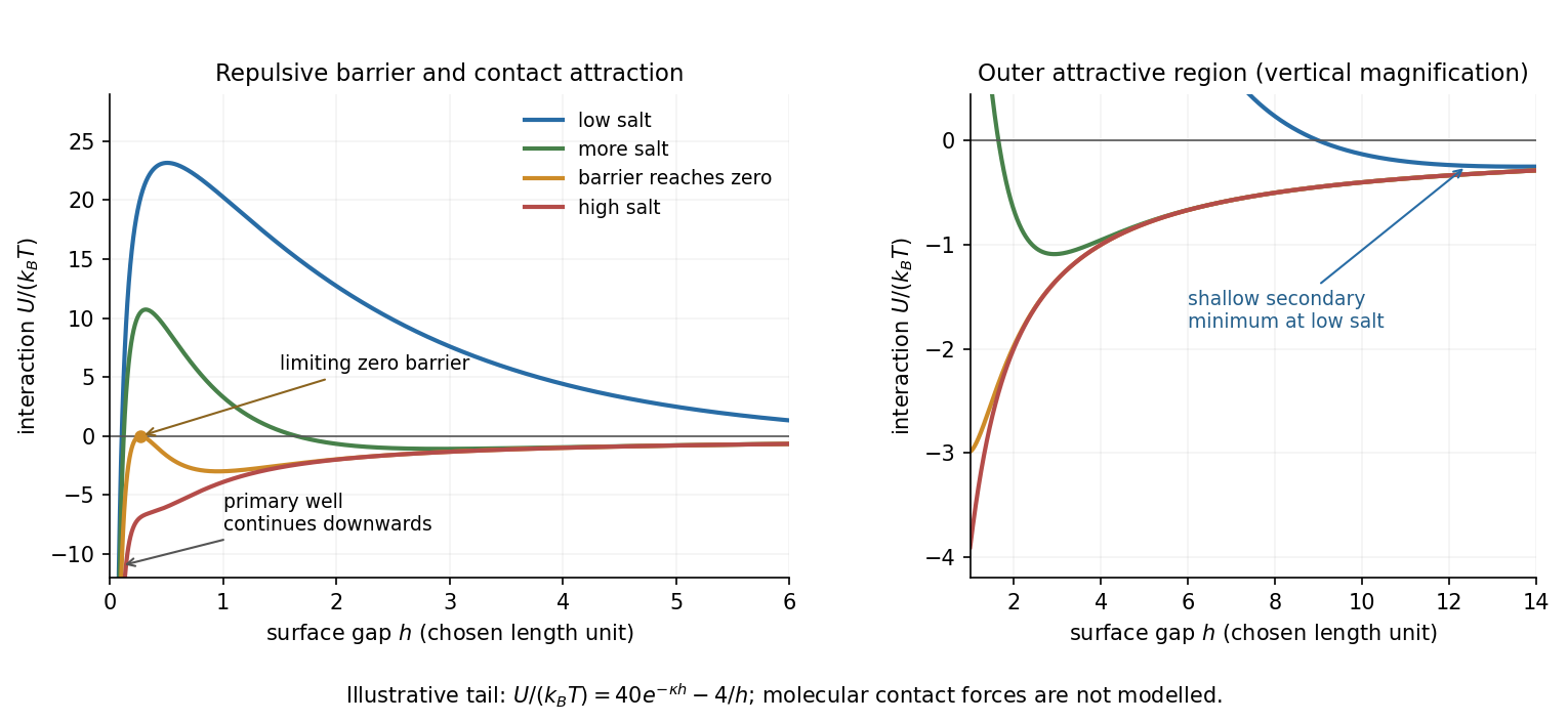
Original schematic DLVO potentials as screening increases
. Illustrative dimensionless amplitudes show the barrier and outer attractive minimum; the near-contact primary well extends below the plotted range. These curves do not determine a material-specific coagulation concentration. Details.
Aggregate structures. Well above the critical coagulation concentration, the sticking probability is close to one. In diffusion-limited cluster aggregation, the first encounter attaches particles or clusters at accessible outer branches before they can explore many alternative configurations. The result is an open, tenuous structure. Typical ideal three-dimensional cluster models have mass fractal dimension .
Near the threshold on its lower-salt, slow-aggregation side, a remaining barrier makes most encounters unsuccessful. Reaction-limited cluster aggregation then permits repeated approaches and orientations before attachment, commonly giving denser clusters with . Since particle count scales as , the larger exponent means more particles at a given large cluster size. This explanation does not require already formed bonds to rearrange: unsuccessful encounters themselves alter which configurations eventually bind.
The side of the threshold matters. At the ideal barrier-free threshold itself, or just above it, aggregation can already be diffusion limited; proximity to the critical coagulation concentration alone does not universally imply a denser reaction-limited structure. The quoted dimensions are typical of irreversible approximately isotropic cluster models, not exact values for every colloid. Strong bond rearrangement or anisotropic attractions can change this comparison.
Oscillatory response. A material with viscoelasticity stores some deformation energy and dissipates some over a loading cycle. In small-amplitude oscillatory shear, represent the strain by . The shear-stress amplitude is related to the strain amplitude by the complex viscoelastic modulusHere is the storage modulus, the component in phase with strain, and is the loss modulus, the dissipative quadrature component. Both have units of pressure. The stress leads the strain by an angle , withFor this convention, a passive material has at positive frequency. Integrating over one period gives dissipated energy per unit volume , and the average input power per unit volume is . Thus the loss tangent compares the dissipative and elastic parts of the response. The frequency dependence reflects which internal relaxation processes can follow the imposed deformation.
Torsional measurement. Use for radial position inside the rod, reserving for its outer radius. A small angular displacement of one end relative to the fixed other end gives shear strainIn harmonic amplitude notation, the shear stress is . Its restoring torque is obtained by multiplying by the lever arm and integrating over the circular section:The factor is the polar second moment of area; it is not the disc's mass moment of inertia . The torsional spring constant becomes the complex stiffness . Angular Newton's second law therefore gives the paper's compact representationIts precise interpretation is a torsional measurement of a complex shear modulus. At a specified frequency, with complex angular amplitude , the driven response obeysSetting the external torque to zero supplies the free-mode condition, whose damped frequencies are generally complex. A dissipative free oscillator does not execute a sustained nonzero oscillation at a real frequency without driving. In real time, a general frequency-dependent complex viscoelastic modulus represents a causal memory response, rather than a complex instantaneous force on a real displacement. The derivation assumes a uniform slender circular rod, small twist, negligible rod inertia relative to the disc, and no additional bending, slip or external damping.
Frequency regimes and sketches. A permanently crosslinked elastomer has a low-frequency rubbery plateau . Slow chain rearrangements can follow the strain, so the network is relatively compliant but still elastic. At high frequency the relevant segmental motions are frozen, giving a much larger unrelaxed or glassy stiffness . Between these regimes the motions lag behind the loading and dissipate strongly.
A standard linear solid model supplies a consistent illustrative sketch of this process. Put , where is the stress viscoelastic relaxation time, and . ThensoAt very low frequency, , and . Through the relaxation region rises, has a maximum and has a loss peak. At high frequency, , and again. Real polymers usually have a spectrum of relaxation times, so these features are broader and can have further structure.
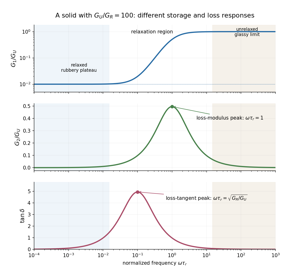

The two kinds of loss peak need not coincide. The peak frequencies in a standard linear solid areThe first follows by differentiating ; the second by differentiating . This is why the sketch marks the peaks separately. If the polymer is an uncrosslinked melt rather than a permanent network, there is an additional ultimate low-frequency terminal-flow regime, with and ; a permanent elastomer does not have that zero-frequency fluid limit.
Interstitial atoms in a metal. A suitable mechanism is the Snoek effect, a form of anelasticity. An interstitial defect distorts its local crystal structure anisotropically. Different site orientations become unequally favorable under an applied stress, so hopping atoms redistribute towards the preferred orientations and supply additional strain. The hopping time is thermally activated, approximately , with activation energy .
At low frequency, , the populations nearly equilibrate during each cycle. The defect contribution to strain is nearly in phase with stress, giving a relaxed compliance and little dissipation. At intermediate frequency, , redistribution lags behind the stress and energy dissipation is largest. At high frequency, , the populations are effectively frozen; the extra relaxation strain cannot develop, and the response approaches the stiffer unrelaxed elastic limit. For weak single-mode relaxation, the loss tangent is approximately proportional to . The metal remains a solid in the low-frequency regime: the extra delayed strain is recoverable, not unrestricted viscous flow.
Ideal and self-avoiding walks. An ideal chain has independent isotropic coarse-grained steps and permits self-intersections in its mathematical model. For steps of length , the cross terms average to zero, so its root-mean-square end-to-end distance of a polymer chain obeysA self-avoiding walk excludes repeated occupancy or intersection at the segment scale. This represents positive excluded volume in a dilute good solvent. The nonlocal constraint correlates otherwise distant portions of the chain and swells it:The Flory approximation replaces this exponent by , by balancing stretching free energy with an interaction contribution . The result is a more extended and less internally dense coil than the ideal walk; self-avoidance changes the statistics, not merely the local step length.
Two ideal-chain regimes. At the theta temperature for a dilute polymer–solvent pair, leading effective segment attractions and repulsions cancel. Large-scale chain statistics are approximately ideal, even though microscopic atoms still have finite size. In a homogeneous polymer melt, surrounding chains screen long-range excluded volume interactions of a chosen chain, again making its equilibrium large-scale size approximately ideal. Local bond-angle correlations must be included in an effective statistical length such as the Kuhn length. Polymer entanglements can slow the dynamics without invalidating this leading equilibrium size law.
Semiflexible DNA. The nucleic acid double helix gives double-stranded DNA a bending stiffness and substantial local orientational persistence. Independent step orientations are therefore a poor description on short scales, while self-avoidance alone does not specify the energy cost of bending. The worm-like chain describes the molecule as a continuously bendable, locally inextensible curve parameterized by arc length , with unit tangent . Its bending energy iswhere is bending stiffness. In the free three-dimensional model, the persistence length is andThus is the contour separation over which tangent alignment falls by the factor ; it quantifies stiffness relative to thermal bending. The model bridges locally rod-like and globally coil-like conformations. It omits long-range self-avoidance in its simplest form, so sufficiently long dilute DNA can require excluded-volume corrections.
Flexible and rigid limits. Integrating the tangent correlation over the two contour positions gives the end-to-end distance of a worm-like chain:For a very flexible chain on the scale of its total length, , the exponential is negligible andThis is the ideal chain result with Kuhn length and effective step count . Many persistent sections have decorrelated orientations. The flexible limit means a large ratio within the continuum model's range, not an extrapolation of the persistence length below all molecular length scales.
For a nearly rigid chain, , the constant and linear terms in the exponential cancel those outside it. The Taylor series givessoThis is the expected rod limit: all tangents are nearly aligned, and the end-to-end distance approaches the arc length.
Helix–coil curves. A helix-coil transition model allows ordered helical runs and disordered coil regions. Use and with exactly the free-energy conventions defined in the paper. A negative gives and favors the helical state; a positive junction cost gives and penalizes starting new domains. The supplied helical fraction is the long-chain form associated with the Zimm-Bragg model.
Its main features follow directly without assuming a sharp transition. Put . For every ,and differentiating givesThus all curves rise monotonically and cross at . Increasing the boundary free-energy cost reduces , suppresses frequent coil–helix boundaries and makes longer runs favorable. The transition region becomes narrower and steeper: balancing against gives a width of order near .
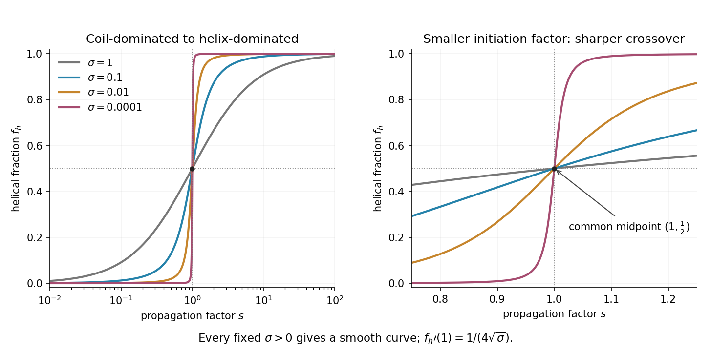

For , the fraction simplifies to , the noncooperative two-state result. For , the steep curve describes cooperative helix formation. In the singular limit , it approaches zero for and one for ; its midpoint remains when approached through positive . Setting directly makes the formula indeterminate at . For any fixed positive , the given long-chain curve is smooth: it is a cooperative crossover, not a true discontinuity. The plot varies at fixed ; in an actual temperature scan both parameters may change, and a finite chain can further round the crossover.
Articles by others on the same topic
There are currently no matching articles.