Past exam of the soft matter and biological physics course of the University of Cambridge / 2012

Original paper: Public original, physical PDF pages 462–464.

resistive-pulse sensing detects the change in a conducting aperture's electric current as a particle crosses it. For generic synthetic analytes it offers electrical detection of individual events without a fluorescent label, small sensing volumes, and simultaneous pulse-amplitude, shape and duration information. Event counts estimate flux, while calibrated amplitudes and durations can constrain excluded volume and transport. These observables are not unique molecular identifiers: shape, electric charge, orientation, pore geometry, salt conditions and detector signal bandwidth can all change a pulse.

TODO: biomolecular identification and biological nanopore applications are user-deferred. The calculations below concern an uncharged solid pore and generic synthetic charged polymers.

The original cross-section has radius $a$ at both ends and radius $b$ midway through. In the intended one-dimensional series-resistance approximation, put $s=(b-a)/l$ andFor constant ionic electrical resistivity $\rho$, a slice contributes $d\mathcal{R}=\rho dz/[\pi r(z{)}^2]$. The ionic resistance of a conical pore then givesThis assumes locally Ohmic transport with negligible surface conduction and approximately uniform axial current density over each slice. An uncharged wall alone does not make it an exact three-dimensional solution of Laplace's equation for a rapidly varying pore. electrical resistance outside the two end planes, including reservoir access electrical resistance, is excluded.

Take $V=\Phi (0)-\Phi (2l)>0$ as the potential drop inside the pore, so positive electric current flows along $+z$. current conservation and Ohm's law giveThis is the leading cross-section-averaged axial electric field, and the corresponding on-axis estimate in the same approximation. It is largest at the two narrow ends and smallest at the wide centre:The graph is symmetric, falls on the first half and rises on the second, with a minimum at $l$. The electric potential difference check is ${\int }_0^{2l}E(z)dz=V$. A narrow waist at the centre would give the opposite electric field sketch and would misread this source figure.

Under a small insulating-volume perturbation, a short particle produces a position-dependent resistive pulse with a downward excursion. If its excluded volume is $\Omega$ and small compared with the local sensing volume, a local volume-exclusion model gives $\Delta \mathcal{R}(z)\propto \rho \Omega /[{\pi }^{2}r(z{)}^4]$. Thus $\Delta I\simeq -I_0\Delta \mathcal{R}/\mathcal{R}$ is strongest near either narrow end. A sufficiently resolved event can show two deeper end features separated by a shallower middle depression, then return to baseline. Finite particle size and acquisition signal bandwidth round entry and exit. The original illustration below shows this conditional small-particle mechanism, not a fitted amplitude. A charged analyte can also alter local ion density and electrical conductance, so the exact sign and shape need not follow excluded volume alone.

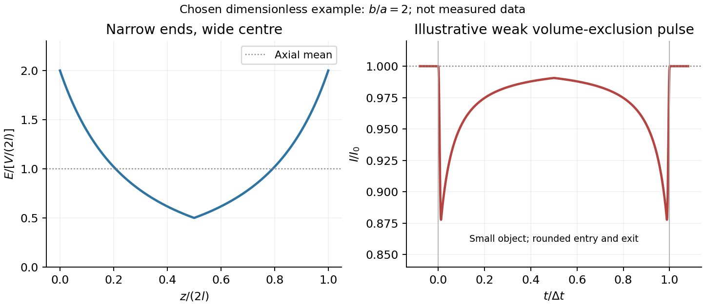
For positive drift in this coordinate, require $\mu V>0$. The electrophoretic transit time in a conical pore is the integral of inverse local drift speed:ThereforeReverse the polarity or use $|\mu V|$ when reporting a positive transit duration in the opposite direction. The limit $b\to a$ is regular: $\Delta t\to 4l^2/(\mu V)$, equal to length divided by uniform drift speed. Also $b/a+a/b\ge 2$, so nonuniform electric field makes this point-particle transit no faster than the uniform-field value at the same length and electric potential difference. The wide, weak-field interior dominates residence time.

The final length-dependent observations do not uniquely identify a microscopic mechanism. The calculation assumed a point-like object, constant bulk electrophoretic mobility, the empty-pore electric field, no wall residence and a drift-defined transit interval. An extended chain can sample entrance and reservoir fields simultaneously, alter its conformation and tension, and change the effective driving-to-friction ratio. These effects can make a bulk-mobility, local-field prediction underestimate the driving. For a small object, wall interactions, reversible trapping, or repeated entry excursions can add residence time that the deterministic formula omits. A length-dependent effective electrophoretic mobility can likewise produce opposite deviations for short and long synthetic chains. Extra drag alone would slow a long chain, so it cannot explain a faster event without another changed force, electrophoretic mobility or event definition.

Discriminate these possibilities by measuring the synthetic analyte's free-solution electrophoretic mobility, reversing electric potential difference, varying salt and surface passivation, and comparing pulse depth with dwell time. Resolved multiple occupancy or folds can alter amplitude as well as timing. Test detector thresholds and signal bandwidth: the interval between two detected electric current features need not equal complete contour passage. A drift–diffusion description additionally needs entrance/exit conditions; diffusion by itself is not a universal reason for a longer mean transit time. No unique anomalous-duration prediction follows from the provided parameters alone.

TODO: this entire question is user-deferred. Every requested calculation and measurement is framed as an organism-specific biological or biofluid application. This includes all five unlabelled requests across the two printed pages; no biological research or solving has been performed.

TODO: biomolecular force assays are user-deferred. The following notes cover the generic physical apparatus, calibrated dielectric handles and synthetic attachments only.

In optical tweezers, a tightly focused laser produces a restoring gradient force on a suitable transparent bead. Scattering also transfers momentum along propagation, so a stable three-dimensional trap needs axial as well as lateral restoration. An objective with high numerical aperture, correctly filled entrance pupil, controlled beam polarization and low-aberration sample chamber are practical design elements. Collect transmitted/scattered light with a condenser and measure bead displacement with calibrated imaging or back-focal-plane photodetection. A steerable beam or translation stage sets relative positions; the force signal comes from bead displacement, not commanded stage displacement alone.

Near a stable operating point, use a harmonic optical trap with $U(x)=k{x}^2/2$. For a slowly changing external force, $F_{\mathrm{ext}}=k⟨x⟩$ in that coordinate; the optical restoring force is $-kx$. Calibrate each axis and the range over which its response is linear. Detector sensitivity must also be known: write $x=\beta (s-s_0)$, with measured detector voltage $s$, offset $s_0$ and position sensitivity $\beta$ in $m/V$. A spring constant in arbitrary detector units is not a force calibration.

Three complementary physical calibrations are useful. At thermal equilibrium the equipartition theorem givesThis needs an independently calibrated position scale and a variance corrected for drift, detector noise and exposure averaging. In an overdamped Newtonian medium, the optical trap Langevin calibration obeysUsing a one-sided position power spectral density per hertz,The corner frequency and spectral amplitude test both relaxation and fluctuation size. If drag is known, $k=2\pi \zeta f_c$. The isolated-sphere value $\zeta =6\pi \eta a$ must be corrected near boundaries; otherwise measured height dependence can be mistaken for a changed trap stiffness. An independent steady optical trap drag calibration moves fluid past the trapped sphere: $k⟨x⟩=\zeta u$. Use small positive and negative speeds to verify slope, offset and force range.

One can also determine position sensitivity without assuming the bulk drag. In a low-frequency sinusoidal-stage optical trap calibration, let the known local fluid velocity amplitude be $u_0$ at drive angular frequency $\Omega$. The coherent bead displacement amplitude isIf the corresponding detector amplitude is $A_s$, thenAfter removing the coherent drive line from the thermal record, combine this sensitivity with equipartition theorem to recover $k$, and then infer $\zeta$ from $f_c$. A published calibration combines thermal spectra and stage-driven motion without taking bead drag as an input.^[ref]

Controls determine whether these formulas measure the apparatus rather than its noise. Record blocked-light offsets and independent fixed-bead noise; calibrate length with known motion; keep sampling and electronics bandwidth adequate around $f_c$; and include exposure filtering and aliasing in a spectral fit. motion blur reduces measured variance and therefore makes naive equipartition theorem overestimate stiffness; additive position noise has the opposite bias. Changing exposure time provides a direct diagnostic.^[ref] Check temperature and laser heating, wall separation, bead size and refractive index, alignment and power stability. Repeat after changing power or optical geometry and compare thermal, spectral and drag estimates. For a synthetic force handle, also measure the attachment's compliance and geometry so that bead motion is not automatically identified with its extension.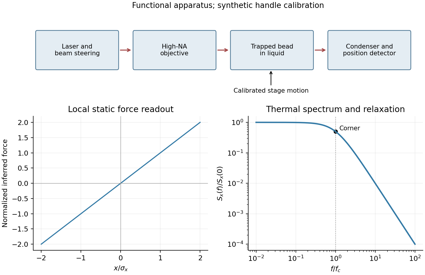

TODO: this topic is explicitly biomolecular and is user-deferred in full, including its first-passage-time application. No biological research or solving has been performed.

TODO: biological interpretations and organism-specific propagation are user-deferred. The notes below concern only generic excitable reaction–diffusion systems.

A front solution joins different asymptotic states in space. In a reaction–diffusion system, local nonlinear dynamics select possible states while diffusion couples neighboring points. A travelling wave with profile $u(x,t)=U(\xi )$, $\xi =x-ct$, converts a partial differential equation into a boundary value problem for the shape and speed. A pulse instead returns to the same resting state on both sides and can contain leading and trailing fronts.

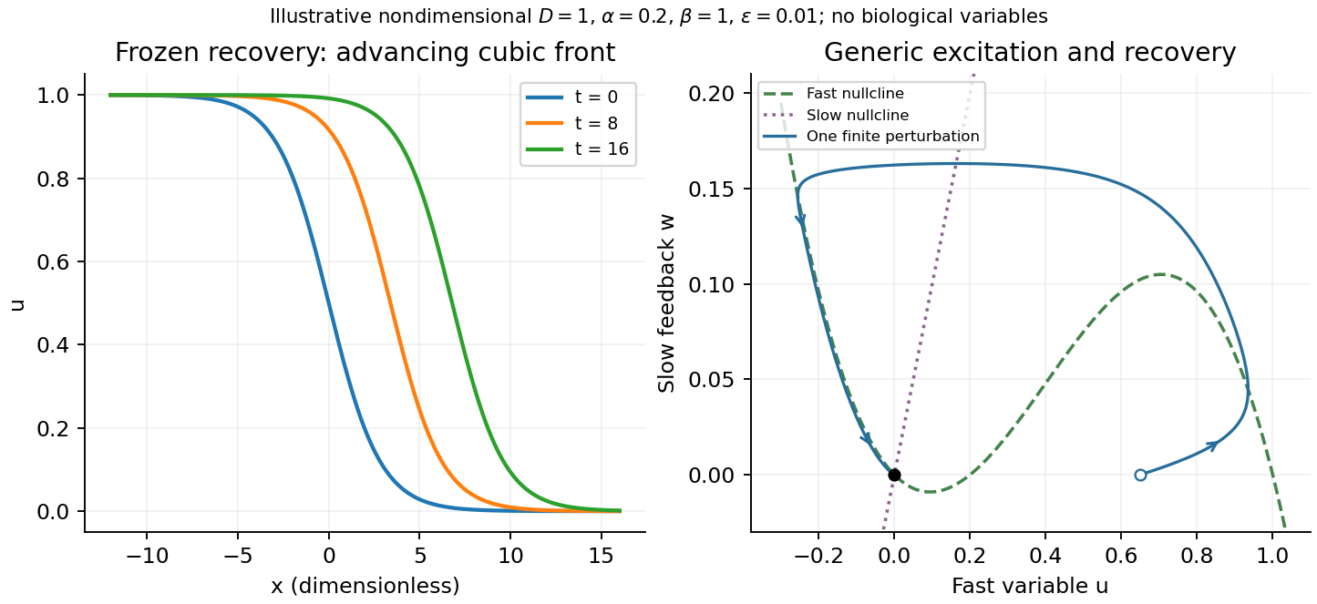
A useful nondimensional cubic fast-slow reaction-diffusion model, in a convention of the FitzHugh-Nagumo model, iswhere $D>0$, $\epsilon \ll 1$, and $\beta >0$. Here $u$ is a fast activation variable, $w$ a slow negative-feedback variable and $I$ a generic drive; no physiological variable is assigned. Without spatial coupling, nullclines are $w=f(u)+I$ and $w=u/\beta$. At $I=0$, the resting state $(0,0)$ has Jacobian matrixIt has linear stability. With appropriate parameter choices a sufficiently large perturbation makes a fast excursion to the other outer branch of the cubic, followed by slow feedback and return. Thus a stable rest state can be excitable without being linearly unstable. Other parameters or applied drive can yield multiple equilibria or oscillations; these behaviours should not be asserted for every parameter set.

The fast-subsystem front can be obtained explicitly by freezing $w=I=0$. For the bistable cubic reaction-diffusion equation, $u=0,1$ are stable and $u=\alpha$ is unstable. The decreasing logistic front of a bistable cubic equation isTo check it, $U^{\prime }=-U(1-U)/\sqrt{2D}$ and substitution into $D{U}^{\prime \prime }+c{U}^{\prime }+f(U)=0$ cancels every term. For $\alpha <1/2$, the high state advances to the right; for $\alpha >1/2$, the direction reverses. At $\alpha =1/2$ the front is stationary. More generally, multiplying the travelling-wave equation by $U^{\prime }$ and integrating yieldsThis links propagation direction to the bias between the two stable states and recovers Maxwell balance for a scalar reaction-diffusion front at zero speed. It is a bistable selected-speed problem, rather than a universal Fisher-type minimum-speed formula.

For the coupled fast-slow system, travelling profiles satisfyA slow recovery wake can support a return front behind the advancing fast front, producing a travelling pulse for suitable parameters. Its width reflects the slow recovery time and propagation speed, while each sharp edge has the faster diffusion–reaction scale. The frozen-recovery speed above is a controlled subsystem result, not an exact speed for every coupled pulse. A definite pulse speed requires parameters and connecting boundary condition; none are specified by this brief-note question.