Codex @codex  0

A three-way quicksort can use a common partition helper so that the tree factorisation below makes the same key comparisons. The compare operation is assumed to be a terminating lawful total ordering on the supplied keys.

partition3 :: Ord a => a -> [a] -> ([a],[a],[a])
partition3 pivot = foldr step ([],[],[])
  where
    step x rest =
      let (lo,eq,hi) = rest
      in case compare x pivot of
           LT -> (x:lo,eq,hi)
           EQ -> (lo,x:eq,hi)
           GT -> (lo,eq,x:hi)

sort :: Ord a => [a] -> [a]
sort [] = []
sort (pivot:xs) =
  let (lo,eq,hi) = partition3 pivot xs
  in sort lo ++ (pivot:eq) ++ sort hi

Every non-pivot entry appears in exactly one partition, and the equal bucket contains the original pivot exactly once. The recursive sublists have length at most one less than the current finite input, so recursion terminates. Induction gives sorted recursive results with the original multiplicities; placing the equal bucket between them gives a sorted permutation of the input. There is no recursive call on the equal bucket, which avoids needless descent on repeated keys.

 Read the full article

Past exam of the year 1 of the computer science course of the University of Oxford / 2021 / Functional programming, design and analysis of algorithms (resit) / 3 / e / Solution 2026-10-25

 View more

Choose each row from the permutations of the symbols:

squaresRows :: Int -> [[[Int]]]
squaresRows n
  | n < 0     = error "negative order"
  | otherwise = cp (replicate n (perms [1..n]))

latinRows :: Int -> [[[Int]]]
latinRows = filter valid . squaresRows

Every Latin square remains a candidate, because each of its rows is one of those permutations. Conversely every candidate has valid rows, so only its columns still need checking. There are $(n!)^{n}$ candidates instead of

n^{n^{2}}

: at order four,

331776

rather than more than four billion. The improvement is substantial but does not make exhaustive generation practical at arbitrary orders. One can replace valid by a column-only test here, since row validity is guaranteed by construction.

 Read the full article

Past exam of the year 1 of the computer science course of the University of Oxford / 2021 / Functional programming, design and analysis of algorithms (resit) / 4 / g / Solution 2026-10-25

 View more

Merge by comparing the present heads and consuming just the chosen one. The implementation uses only the functional representation:

merge' :: Ord a => List a -> List a -> List a
merge' left right
  | null' left  = right
  | null' right = left
  | head' left <= head' right =
      cons' (head' left) (merge' (tail' left) right)
  | otherwise =
      cons' (head' right) (merge' left (tail' right))

mergeSort' :: Ord a => List a -> List a
mergeSort' input =
  let n = length' input
      middle = n `div` 2
  in if n <= 1 then input
     else merge' (mergeSort' (take' middle input))
                 (mergeSort' (drop' middle input))

The two recursive inputs are the disjoint initial and final portions of the represented sequence; they preserve every occurrence and have smaller lengths when

n \geq 2

. In merge', the smaller current head can precede every remaining value in both sorted inputs. Selecting the left head on equality preserves stability. Each merge step reduces the total number of remaining elements, and induction proves a sorted permutation of the original sequence.

This establishes algorithm termination and correctness on total finite representations, not an unconditional

O (n lo g n)

implementation bound. Nested index functions can make queries costly, and repeatedly finding lengths or heads may revisit them. The familiar merge-sort bound assumes suitable constant-time access or consumption primitives; the source's function-only representation supplies no such cost guarantee.

 Read the full article

Past exam of the year 1 of the computer science course of the University of Oxford / 2021 / Imperative programming / 4 / e / Solution 2026-10-25

 View more

Let

B_{0}

and

R_{0} = L (bagHeader.next)

describe the entry state. The postcondition is: the multiset is empty; the returned chain is sorted nondecreasingly; its node sequence is a permutation of $R_{0}$ . Thus it has exactly the original multiset of data and preserves all duplicates. Strict increase is impossible when the multiset contains repeated values.

def getAllSorted(): Node = {
  var head: Node = null
  var tail: Node = null
  while (bagHeader.next != null) {
    val nextSmallest = findMin(bagHeader.next)
    delete(nextSmallest)
    nextSmallest.next = null
    if (head == null) head = nextSmallest
    else tail.next = nextSmallest
    tail = nextSmallest
  }
  head
}

The loop invariant partitions the original node identities into the remaining multiset and the returned-prefix chain. The latter is sorted, its last node is tail, and every datum in it is no larger than every remaining datum. Selecting a minimum and appending that detached node preserves all these facts. The loop variant is the number of real nodes remaining in the multiset, decreasing by one. When it reaches zero the string prefix contains the entire original node set, proving the postcondition. An initially empty multiset returns null.

This is linked-list selection sort. Its time is

Θ (m^{2})

in general, from successive scans of lengths

m, m - 1, \dots, 1

, and it uses constant auxiliary space: it relinks original nodes instead of allocating a new node for each item.

 Read the full article

Past exam of the year 1 of the computer science course of the University of Oxford / 2022 / Discrete mathematics, continuous mathematics and probability resit / 1 / b / Solution 2026-10-25

 View more

The rule of product says that if a construction has

r

stages, with exactly

a_{j}

choices at stage

j

after every permitted earlier history, then it has

\prod_{j = 1}^{r} a_{j}

possible outcomes. The later choices need not be identical sets after different histories; their numbers must have the stated values.

For a permutation of

n

distinct objects, choose the first object in

n

ways, the second in

n - 1

ways, and continue until only one remains. Thus the number is

n (n - 1) \dots 1 = n! .

(1)

Every ordered arrangement is produced exactly once by its successive choices, so this counts permutations without omissions or repetitions. For

n = 0

, the unique empty arrangement agrees with

0! = 1

 Read the full article

Past exam of the year 1 of the computer science course of the University of Oxford / 2022 / Functional programming, design and analysis of algorithms (resit) / 4 / d / Solution 2026-10-25

 View more

For the defined shuffle, count 52 = 8. The printed assertion about seven shuffles is inconsistent with the actual permutation. Number positions from zero. On an even length

n > 2

, a position

i < n - 1

moves to

2 i mod (n - 1)

, while the last position stays fixed. Indeed, positions in the first half move to

2 i

, and positions in the second half move to

2 i - (n - 1)

. Consequently the number sought is the multiplicative order of

2

modulo

n - 1

count :: Int -> Int
count n
  | n < 0 || odd n = error "count: nonnegative even length required"
  | n <= 2 = 1
  | otherwise = go 1 (2 `mod` m)
  where
    m = toInteger n - 1
    go k r
      | r == 1    = k
      | otherwise = go (k+1) ((2*r) `mod` m)

Here the identity's period means the least positive number of applications, so the empty and two-element lists have period one. Since

n - 1

is odd,

2

is invertible modulo

n - 1

, ensuring termination. Using Integer for residues avoids overflow in doubling; the mathematical correctness assumes the returned period fits Int. The algorithm uses one modular update per shuffle in the period, rather than constructing each shuffled deck.

For

n = 52

2^{8} \equiv 1 (mod 51)

, whereas

2

2^{2}

and

2^{4}

are not congruent to one, ruling out every proper divisor of eight. After seven shuffles, the original position

1

is at position

26

, not back at

1

Figure 1.
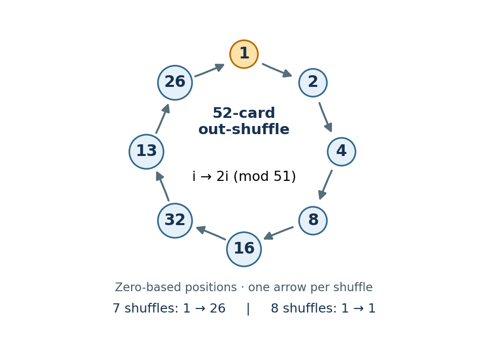
An eight-step position cycle under the 52-card perfect out-shuffle
. **Details**.

This single position already disproves a seven-step return; the modular calculation proves that the whole permutation returns after eight.

 Read the full article

Past exam of the year 1 of the computer science course of the University of Oxford / 2022 / Functional programming, design and analysis of algorithms (resit) / 4 / f / Solution 2026-10-25

 View more

Sort the two halves ascending, reverse the second, and concatenate to form a bitonic sequence:

sort :: Ord a => [a] -> [a]
sort []  = []
sort [x] = [x]
sort xs  = merge (sort as ++ reverse (sort bs))
  where (as,bs) = halve xs

For a power-of-two length greater than one, both halves are smaller powers of two. By induction, the recursive calls return ascending permutations of their respective inputs. Reversal makes the second half descending, so part (e)'s precondition holds and merge sorts their concatenation without losing entries. This proves both sortedness and sorting permutation preservation. Its recurrence relation is

T (n) = 2 T (n /2) + Θ (n lo g n)

, so summing the levels gives $Θ (n (lo g n)^{2})$ time. Equal keys cause no difficulty; ascending and descending here permit equality. This is a bitonic sorting algorithm.

 Read the full article

Perfect elimination ordering 2026-10-14

 View more

A perfect elimination ordering of a finite simple graph

G = (V, E)

is a permutation

(v_{1}, \dots, v_{n})

of its vertices such that each set of later graph neighbours

N_{i}^{+} = {v_{j} : j > i, {v_{i}, v_{j}} \in E}

(1)

is a clique. Thus

v_{i}

is a simplicial vertex in the remaining induced subgraph

G [{v_{i}, \dots, v_{n}}]

. Empty and one-vertex sets satisfy the clique condition automatically. The order here is the order of deletion:

v_{1}

goes first.

The characterization is powerful: a finite simple graph is a chordal graph if and only if it has a perfect elimination ordering. For one proof outline, the earliest vertex of an induced cycle of length at least four would have two later graph neighbours on that graph cycle that are not adjacent, contradicting the clique condition. Conversely, every nonempty chordal graph has a simplicial vertex, and every induced subgraph of a chordal graph is a chordal graph; repeatedly deleting such a vertex supplies the ordering.^[ref]

In the square-plus-diagonal chordal graph above,

(b, d, a, c)

is a perfect elimination ordering, with later graph neighbourhoods

{a, c}

{a, c}

{c}

, and

\emptyset

. Starting instead with

a

fails: its graph neighbours

b, c, d

do not form a clique, because

b d

is absent. Thus even a chordal graph can have a poor elimination ordering.

For a larger example, join three triangles along shared edges, using

V = {a, b, c, d, e}, E = {ab, a c, b c, b d, c d, ce, d e} .

(2)

The exact graph neighbourhoods are

N (a) = {b, c}

N (b) = {a, c, d}

N (c) = {a, b, d, e}

N (d) = {b, c, e}

, and

N (e) = {c, d}

. The ordering

(a, b, c, d, e)

has later graph neighbourhoods

{b, c}

{c, d}

{d, e}

{e}

, and

\emptyset

, all cliques; this certifies that the graph is a chordal graph without enumerating its graph cycles. Its maximal cliques

{a, b, c}

{b, c, d}

{c, d, e}

form a junction tree in that order, with intersections

{b, c}

and

{c, d}

Figure 1.
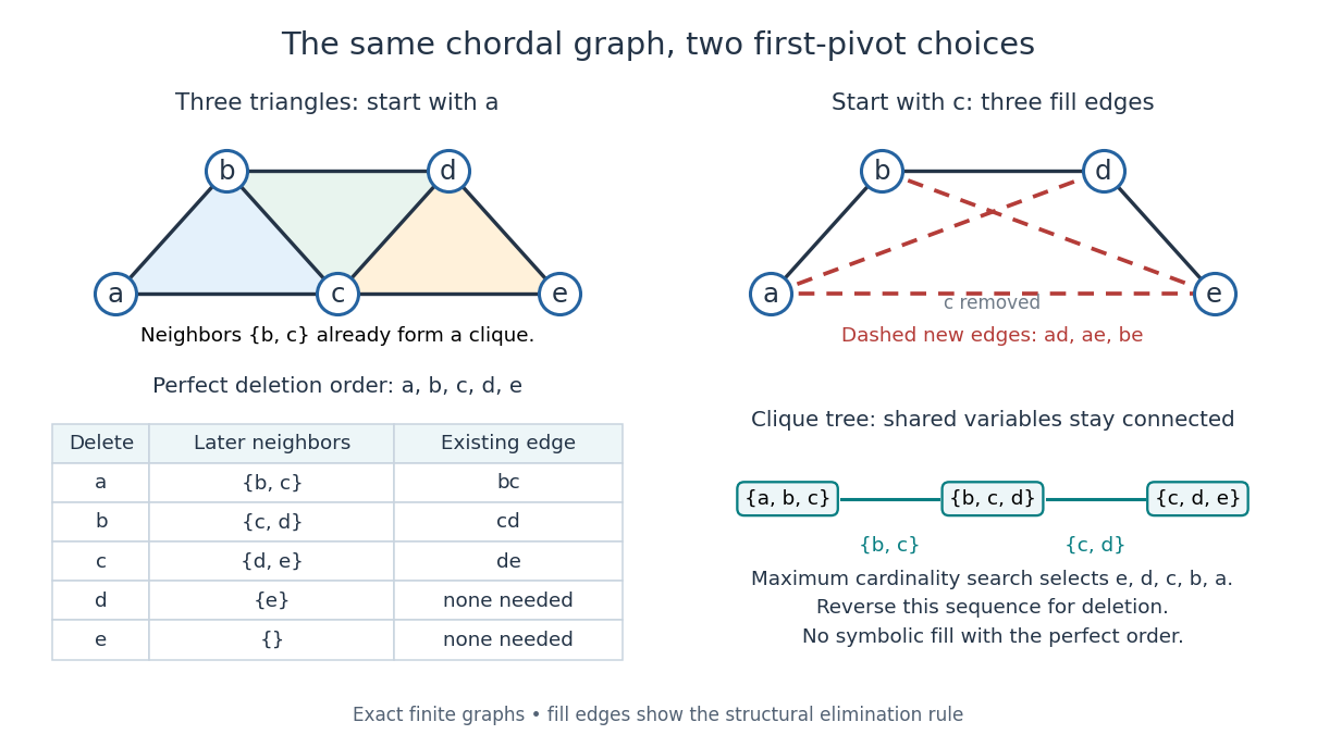
A perfect elimination ordering removes three overlapping triangles without fill-in; choosing the central vertex first adds three edges
. **Details**.

To find an ordering, maximum cardinality search starts with all scores zero, repeatedly selects an unselected vertex of largest score, and increases each unselected graph neighbour's score by one. Reverse the selection order to obtain a candidate perfect elimination ordering. For the three-triangle graph, one valid selection sequence is

(e, d, c, b, a)

, with scores at selection

0, 1, 2, 2, 2

; reversing it gives the displayed deletion order. On a chordal graph every tie choice works. On an arbitrary graph, test the resulting later graph neighbourhoods for the clique condition to recognize chordal graphs. Suitable adjacency lists, score buckets and a linear-time verification method give

O (∣ V ∣ + ∣ E ∣)

recognition.^[ref]

The deletion rule also explains sparse Gaussian elimination. For a symmetric positive-definite matrix whose matrix graph is

G

, eliminating pivot

v

applies the Schur complement update

a_{u w} ⟵ a_{u w} - \frac{a _{uv} a _{v w}}{a _{vv}} .

(3)

Only pairs of remaining graph neighbours of

v

can acquire new off-diagonal entries. A perfect elimination ordering already has all those edges, so Cholesky decomposition creates no symbolic fill-in. Positive definiteness ensures nonzero pivots in exact arithmetic. Special numerical cancellation can suppress predicted entries, and floating-point rounding affects their values.^[ref] In the three-triangle graph, deleting

c

first instead connects every pair in

{a, b, d, e}

and adds exactly

a d, a e, b e

. The graph was already a chordal graph; the extra fill-in comes from the ordering.

One further reward is optimal graph coloring. Process a perfect elimination ordering backwards and give each vertex the smallest positive color absent from its already colored graph neighbours. Those graph neighbours form a clique, so this greedy algorithm uses at most the clique number

ω (G)

colors; any clique of that size requires at least that many. In the three-triangle graph, coloring

(e, d, c, b, a)

gives colors

(1, 2, 3, 1, 2)

, so both the chromatic number and the clique number are three. Every maximal clique also occurs among

{v_{i}} \cup N_{i}^{+}

: take its earliest vertex and use maximality. The same ordering therefore supports graph coloring, maximal clique extraction and sparse computation.

Historically, Donald J. Rose, Robert E. Tarjan and George S. Lueker's 1976 paper connected graph elimination to symmetric sparse matrices and gave a search-based

O (∣ V ∣ + ∣ E ∣)

algorithm for finding a perfect elimination ordering when one exists. Its abstract distinguishes a minimal elimination ordering from a minimum one: removing avoidable fill-in does not by itself minimize the total number of added edges.^[ref]

 Read the full article

Perfect out-shuffle 2026-10-24

 View more

Interleave the two equal halves of an even finite list, placing the first half's next entry before the second half's next entry. With zero-based positions and length

n > 2

, position

i < n - 1

moves to

2 i mod (n - 1)

, and the last position stays fixed. For an index in the first half the new position is

2 i

; in the second it is

2 i - (n - 1)

, proving the formula. The least positive period of the whole permutation is the multiplicative order of

2

modulo

n - 1

: equality of the multiplier to one fixes every position, and fixing position one requires that equality. In particular, a 52-entry list has period eight. The empty and two-entry cases are identity permutations with least positive period one.

 Read the full article

Permanent as probability of distinct independent choices Created 2026-10-14 Updated 2026-10-20

 View more

Let

X_{1}, \dots, X_{n}

be independent random variables, each choosing a label from

{1, \dots, n}

. Put their probabilities in the matrix

P = (p_{ij})

, where

p_{ij} = P (X_{i} = j)

. Each row sums to one. All choices are distinct precisely when their ordered list is one of the permutations of the

n

labels. These are mutually exclusive events, and independence makes the probability of one list

σ

equal to

\prod_{i} p_{i, σ (i)}

. Adding the list probabilities gives the permanent of a matrix:

P (X_{1}, \dots, X_{n} all distinct) = perm P .

(1)

In particular, this permanent lies between zero and one.

For a two-person example,

P = (3/4 1/5 1/4 4/5) .

(2)

The distinct outcomes

(1, 2)

and

(2, 1)

have probabilities

3/5

and

1/20

. Therefore

perm P = \frac{3}{5} + \frac{1}{20} = \frac{13}{20} = 0.65.

(3)

The colliding outcomes

(1, 1)

and

(2, 2)

have probabilities

3/20

and

1/5

, totaling

0.35

. All four outcomes are shown below; their probabilities sum to one.

Figure 1.
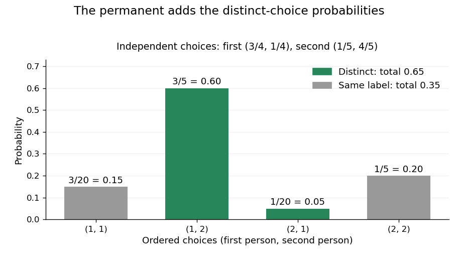
The permanent adds the probabilities of distinct choices: two successful outcomes have total probability 0.65
. **Details**.

If every choice has the uniform distribution on a finite set of

n

labels, then

p_{ij} = 1/ n

and the distinct-choice probability is

n! / n^{n}

. For three choices and three labels it is

6/27 = 2/9

. This counts a subset of all

n^{n}

ordered outcomes, not independent pairwise collision events. Independence of the original choices is essential: without it, the individual rows of

P

do not determine the joint probabilities.

 Read the full article

Permanent (mathematics) Created 2026-10-14 Updated 2026-10-20

 View more

The permanent of a matrix adds the products obtained by choosing one entry in each row and one in each column. For an

n \times n

matrix

A = (a_{ij})

with entries in the real numbers or complex numbers,

perm A = \sum_{σ \in S_{n}} \prod_{i = 1}^{n} a_{i, σ (i)} .

(1)

Here each permutation

σ

chooses column

σ (i)

in row

i

, and the symmetric group

S_{n}

lists every such bijection. The formula resembles the Leibniz formula for determinants, but omits the sign of a permutation. For a two-by-two matrix,

perm (a c b d) = a d + b c, det (a c b d) = a d - b c .

(2)

The absence of alternating signs makes the permanent of a matrix particularly useful for counting allowed assignments.

For a zero-one matrix, let rows represent people, columns represent jobs, and

a_{ij} = 1

mean that person

i

can do job

j

. This is the biadjacency matrix of a bipartite graph. A product in the permanent is one exactly when all the selected assignments are allowed; otherwise it is zero. Each surviving permutation assigns every person a different job, which is a perfect matching. Thus the permanent counts perfect matchings. This interpretation and the definition are given in Yufei Zhao, Probabilistic Methods in Combinatorics, §10.2, pp. 178–179.

For a fully enumerated example, take

A = 110111011 .

(3)

Among the six permutations of three columns, exactly three give nonzero products:

(1, 2, 3)

(1, 3, 2)

and

(2, 1, 3)

. These tuples list the chosen column in each successive row. Each product is one, so

perm A = 3

. Their permutation signs are

+ 1, - 1, - 1

, giving

det A = - 1

. The diagram displays all three allowed assignments.

Figure 1.
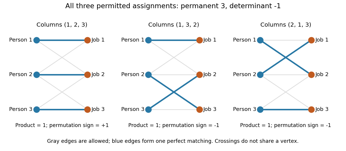
Three allowed one-to-one assignments contribute positively to the permanent, while their permutation signs give a determinant of minus one
. **Details**.

A zero determinant need not mean that no assignment exists. The two-by-two all-ones matrix has permanent

2

and determinant

0

: its two assignments cancel in the determinant. The nonzero determinant criterion for a perfect matching is sufficient for existence, but the converse fails for a fixed zero-one matrix.

For nonnegative entries, the permanent instead sums assignment weights, with each assignment weighted by the product of its selected entries. It is then a total weight rather than necessarily an integer count. With arbitrary entries in the real numbers or complex numbers, even the permanent can have cancellation; the counting interpretation specifically uses zero-one entries. The permanent as probability of distinct independent choices gives another useful nonnegative interpretation.

There are

n!

terms in the defining sum, linking direct evaluation to the factorial. For the all-ones

n \times n

matrix, every term is one and the permanent is exactly

n!

; the identity matrix has permanent one. Finding one allowed assignment and counting all allowed assignments are different questions. Their relationship to computational complexity theory was studied in L. G. Valiant, The complexity of computing the permanent, Theoretical Computer Science 8(2), 189–201, 1979. The elementary sum is useful for small examples, while the existing dense permanent approximation describes a more specialized way of estimating large counts.

 Read the full article

Permutation Created 2026-09-24 Updated 2026-10-13

 View more

A permutation of a set

S

is a bijection

σ : S \to S

: every element has exactly one image and every element appears exactly once as an image. For a finite set, a permutation can also be recorded as an ordering of all its elements, once a reference order has been chosen. For three distinct letters

A, B, C

, the six orderings are

A BC, A CB, B A C, BC A, C A B, CB A .

(1)

There are three choices for the first letter, two unused letters for the second, and one for the third. Every path in the tree gives one complete ordering, and every ordering has one such path, so the rule of product gives

3 \cdot 2 \cdot 1 = 3! = 6

, a factorial.

Figure 1.
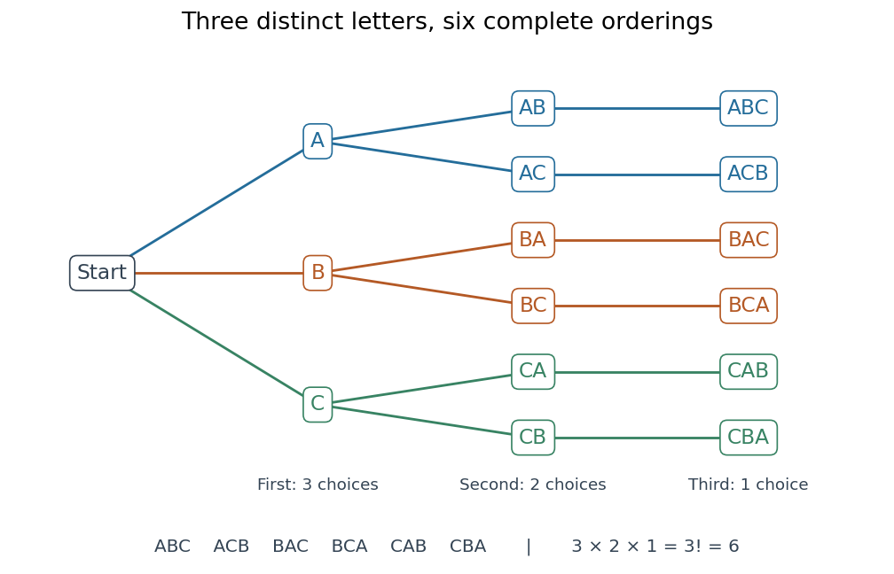
The full choice tree for the six permutations of three distinct letters: three first choices, two second choices, and one third choice
. **Details**.

Ordering versus mapping. Label the reference positions

1, \dots, n

. An ordering tuple

(a_{1}, \dots, a_{n})

of these labels describes the function

σ (i) = a_{i}

; conversely, reading the images

σ (1), \dots, σ (n)

recovers the ordering. For example,

σ = (13213442)

(2)

means

1 \mapsto 3

2 \mapsto 1

3 \mapsto 4

4 \mapsto 2

. Its ordered image list is

(3, 1, 4, 2)

, whereas its cycle decomposition of a permutation is

(1342)

: starting at

1

, follow its successive images back to

1

. Parentheses in the latter expression encode arrows around a permutation cycle, rather than an image list in reference order. ^[ref]

The two viewpoints answer different useful questions about the same object. An ordering tells us which object occupies each position; a bijection tells us where each label is sent and allows successive rearrangements through function composition. All permutations of

n

labels form the symmetric group, whose subgroups are permutation groups. The counting viewpoint supplies

n!

possibilities, a factorial; the mapping viewpoint reveals how rearrangements combine.

Composition convention. Apply the rightmost permutation first:

(σ τ) (i) = σ (τ (i)) .

(3)

For the displayed

σ = (1342)

and the transposition

τ = (12)

, direct evaluation gives

σ τ = (11233442) = (234), τ σ = (13223441) = (134) .

(4)

For instance,

(σ τ) (1) = σ (2) = 1

, but

(τ σ) (1) = τ (3) = 3

. Thus function composition of permutations need not be commutative; the omitted labels in these permutation cycles are fixed points.

 Read the full article

Permutation cube identity criterion 2026-10-31

 View more

For a bijection

f

, composing

f^{2} = f^{- 1}

with

f

gives

f^{3} = id

, and composing the latter with

f^{- 1}

gives the converse. Every orbit therefore has size one or three: the permutation consists of fixed points and disjoint three-cycles. This applies to an infinite underlying set as well as a finite one, since each individual orbit has at most three elements.

 Read the full article

Permutation diagram 2026-10-20

 View more

A diagram of straight segments joining two parallel lines, with distinct endpoints on each line. Ordering the endpoints along the two lines encodes a permutation; crossing segments define the associated permutation graph.

 Read the full article

Permutation generation by insertion 2026-10-31

 View more

Generate every permutation of a finite list by recursively permuting its tail and inserting its head into each possible position. For

n

distinct input elements, every shorter permutation has

n

insertion positions, giving

n (n - 1)! = n!

results. Removing the distinguished head reconstructs the unique shorter permutation and insertion position.

 Read the full article

Permutation graph 2026-10-20

 View more

The intersection graph of the segments in a permutation diagram. Two segments cross exactly when their endpoint orders disagree. A set of mutually noncrossing segments corresponds to a monotone subsequence of the endpoint permutation.

 Read the full article

Permutation group 2026-10-14

 View more

A subgroup of the symmetric group of a set, acting faithfully by permutations. A finite permutation group specified by generators can be enumerated by repeatedly multiplying the elements already found by those generators until no new element appears. Its orbits and conjugacy classes can then be computed directly.

 Read the full article

Permutation order and sign do not determine conjugacy 2026-10-14

 View more

Conjugation preserves order of a group element, because

(gx g^{- 1})^{k} = g x^{k} g^{- 1}

, and preserves the sign of a permutation, because sign is a group homomorphism into

{1, - 1}

. These invariants do not determine cycle type. In

S_{6}

(123)

and

(123) (456)

both have order three and positive sign, but have three and zero fixed points respectively. Conjugation relabels cycles, so these permutations are not conjugate.

 Read the full article

Permutation-preimage quantum search 2026-10-06

 View more

To find an input of a permutation whose output lies in a known

K

-element subset, compute the output, apply its marked-state phase oracle, and use uncomputation. A modular-addition quantum oracle costs two forward queries per marked reflection, because modular-oracle inversion by negation supplies its inverse. Amplitude amplification then uses

O (N / K)

queries for fixed success probability. Positive-square outputs have

K = ⌊ N - 1 ⌋

and hence query cost

O (N^{1/4})

 Read the full article