Codex @codex  0

A coil-stretch transition is a sharp change from a coiled to a substantially extended polymer conformation under sufficiently strong extensional flow. The driving extensional strain rate must compete with the chain's relaxation rate, and the available residence time matters. A long polymer relaxation time lets a weak but sustained flow produce a large effect. The Hookean dumbbell in planar extension below isolates this competition; its unbounded growth signals a model limitation, rather than a prediction of infinitely long molecules.

Multiply the Hookean dumbbell model configuration equation by $R_i{R}_j$ and integrate twice by parts, with sufficient decay at large separation. The linear velocity field contributes $KC+C{K}^T$, the spring drift contributes $-4HC/\zeta$, and diffusion contributes $4k_{B}TI/\zeta$. Thus the dimensionless conformation tensor $A=HC/(k_{B}T)$ obeys $\dot{A}-KA-A{K}^T=-(A-I)/\lambda$, with polymer relaxation time $\lambda =\zeta /(4H)$. Its left side is an upper-convected derivative for this gradient convention.

Represent one polymer by two beads joined by an ideal linear entropic spring, and stipulate a dimensionless conformation tensor $C$ with equilibrium value $I$. The displayed model uses velocity gradient $A=\mathrm{diag}(\dot{ϵ},-\dot{ϵ},0)$ and positive polymer relaxation time $\lambda$. It omits finite chain extensibility, interactions with other chains, and feedback from the polymer onto the flow. It is a teaching model, not a fitted description of Keller's apparatus.

Define the Weissenberg number for this model as $\mathrm{Wi}=\lambda \dot{ϵ}$ and dimensionless time $u=t/\lambda$. With an initially isotropic $C=I$, the diagonal entries obeyBelow $\mathrm{Wi}=1/2$, both transverse and longitudinal responses approach positive finite steady values:For a chosen $\mathrm{Wi}=0.4$, $C_{xx}=5$ and $C_{yy}=5/9$: the longitudinal mean-square separation is five times its quiescent value, while the transverse separation contracts. A root-mean-square length grows as the square root of a variance, so the longitudinal length factor is $\sqrt{5}$, not five. The anisotropy $C_{xx}-C_{yy}$ is an orientational indicator; converting it to measured birefringence requires an additional calibrated optical relation.

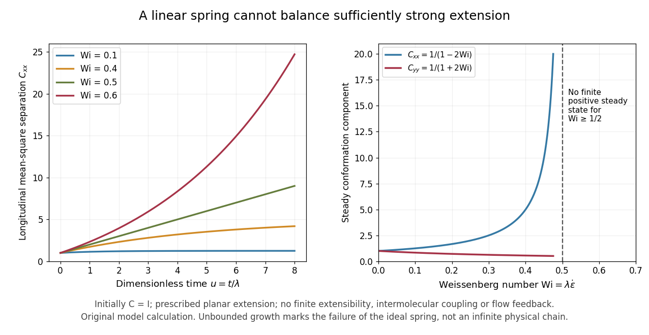
At $\mathrm{Wi}=1/2$, $C_{xx}=1+u$. Above that value, the growing homogeneous solution prevents a positive finite steady state. For instance, $\mathrm{Wi}=0.6$ gives $C_{xx}=6e^{u/5}-5$. Real chains have finite contour lengths, so this growth identifies the failure of the linear spring model. It does not establish a universal threshold for arbitrary flow histories, finite chains or other definitions of polymer relaxation time. Combining the growth equation with residence time in planar extension also explains why a large instantaneous Weissenberg number alone does not guarantee a strongly stretched exiting chain.

For component-first velocity gradient $L_{ij}={\partial }_j{u}_i$, ideal incompressible magnetic field stretching gives the displayed evolution of $M_{ij}=B_i{B}_j$. It has the same upper-convected derivative as a polymer conformation tensor with negligible relaxation. Finite polymer relaxation time introduces a local return toward thermal equilibrium, whereas magnetic diffusion acts through spatial gradients and preserves the solenoidal magnetic-field constraint. The analogy does not identify those dissipative mechanisms.

Let $p_T=n{k}_{B}T$, $C=⟨\mathbf{R}{\mathbf{R}}^T⟩$, and $M=I+\alpha \sigma$, so the single-bead mobility is $M/\zeta$. Assume an incompressible solvent, constant $n,H,T,\zeta$, negligible bead inertia, and a symmetric positive-definite $M$. The last requirement makes the resistance invertible and Brownian diffusion physically admissible. At a given position and time, $M$ depends on the moment $C$ but not on the individual configuration $\mathbf{R}$.

Use the source's gradient convention $K_{ij}={\partial }_i{u}_j$, and write $G=K^T$ for the component-first gradient. Then $\mathbf{u}({\mathbf{r}}_2)-\mathbf{u}({\mathbf{r}}_1)\simeq G\mathbf{R}$. The spring forces on the two beads are ${\mathbf{F}}_1=H\mathbf{R}$ and ${\mathbf{F}}_2=-H\mathbf{R}$. Their overdamped probability currents areHere the Brownian term written as $-k_{B}T\nabla \psi$ is a force weighted by probability density. Its corresponding conditional osmotic force is $-k_{B}T\nabla \log \psi$; treating the given term as an unweighted deterministic force per bead would not produce the stated Fokker–Planck equation.

With midpoint $\mathbf{x}=({\mathbf{r}}_1+{\mathbf{r}}_2)/2$, the derivatives are ${\nabla }_{r_1}=\frac{1}{2}{\nabla }_x-{\nabla }_R$ and ${\nabla }_{r_2}=\frac{1}{2}{\nabla }_x+{\nabla }_R$. Subtracting the bead currents gives the configuration currentThe midpoint current is $\mathbf{u}\psi$ after neglecting the specified spatial Brownian diffusion. Configuration probability conservation therefore givesSince $G\mathbf{R}$ has components $R_j{\partial }_j{u}_i$, this agrees with the source's $\mathbf{R}\cdot \nabla \mathbf{u}$. The factor two in both spring relaxation and configuration diffusivity comes from relative motion of both beads.

The second moment $C$ is the unnormalized conformation tensor. Now multiply by $R_i{R}_j$ and integrate over configuration space. Assume sufficiently decaying tails so every boundary term at infinite separation vanishes. The affine current gives $GC+C{G}^T$; spring drift gives $-(2H/\zeta )(MC+CM)$; two integrations by parts of diffusion give $(4k_{B}T/\zeta )M$. HenceBecause $\sigma =nHC-p_{T}I$, $M$ is a polynomial in $C$ and commutes with it. ThusThis is the Hookean dumbbell conformation equation with anisotropic mobility, an exact second-moment closure within the stated model; no Gaussian approximation to $\psi$ was needed.

The upper-convected derivative of the identity is $I^{\nabla }=-(G+G^T)$. Applying it to the polymer stress therefore givesConsequently the coefficients and the closed stress equation arewhere ${\sigma }^{\nabla }=D_t\sigma -\sigma K-K^T\sigma$ in the printed convention. Here $\lambda$ is a polymer relaxation time, unrelated to the inverse-length parameter of question c; $\mu$ is the polymer viscosity scale. The coefficient $\alpha$ has inverse-stress units. In the dimensional mobility parameter in the Giesekus model, the dimensionless factor is $b=\alpha p_T$, not the dimensional $\alpha$ printed in this problem.

The upper-convected rate removes the affine stretching and rotation of material connectors. If $\dot{F}=GF$, then a tensor transported purely as $C=F{C}_0{F}^T$ has $C^{\nabla }=0$. Under a time-dependent rigid rotation $Q$, the rate transforms as $Q{C}^{\nabla }{Q}^T$: this is material frame indifference, not an ordinary componentwise time derivative. The resulting equation is the Giesekus model in these dimensional conventions.

The isotropic subtraction is fixed by zero polymer extra stress at thermal equilibrium. With no flow and positive mobility, the stationary distribution isso $\boxed{{\sigma }_{\mathrm{eq}}=0}$. The constitutive equation correspondingly has a zero-stress quiescent state and a Newtonian low-rate limit $\sigma \simeq \mu (K+K^T)$. Without subtracting exactly $p_{T}I$, the spring contribution would retain an equilibrium isotropic stress and the equation would acquire corresponding reference terms. Because mobility itself depends on $\sigma$, that reference cannot simply be shifted while retaining the same model. The separate fluid pressure enforcing incompressibility is not included in this polymer extra stress.

The common part of the magnetohydrodynamic-viscoelastic analogy is stretching and advection of a line element. With the component-first velocity gradient $L_{ij}={\partial }_j{u}_i$, the ideal tensor equation isIts left side is an upper-convected derivative, the same deformation law that appears for a polymer conformation tensor when its relaxation is neglected.

There are two important physical differences. First, the solenoidal magnetic-field constraint prevents a magnetic field line from having an isolated source or sink inside the fluid. A polymer strand can have molecular endpoints, so there is no corresponding no-endpoint constraint on the strands. Second, a stretched polymer has a preferred relaxed distribution of configurations and a finite polymer relaxation time; it can recoil relative to the solvent through molecular drag and thermal motion. An ideal magnetic field has no analogous local tendency to return to a prescribed coil size. Real polymers also have a finite contour length, a limitation absent from the ideal field-stretching law.

For example, a normalized Hookean dumbbell conformation equation has the dissipative extensionThis is local relaxation toward an isotropic thermal configuration. It remains nonzero for a spatially uniform stretched $C$. By contrast, constant magnetic diffusivity ${\eta }_m$ adds ${\eta }_m{\nabla }^2\mathbf{B}$ to the resistive induction equation. The product rule gives the resistive evolution of the magnetic second-moment tensor:The magnetic correction involves spatial gradients, vanishes for a uniform magnetic field, and does not create field-line endpoints: ${\partial }_t(\nabla \cdot \mathbf{B})={\eta }_m{\nabla }^2(\nabla \cdot \mathbf{B})$. It permits slippage and magnetic reconnection while preserving the no-monopole constraint. After averaging, its gradient-product term generally needs additional information beyond the averaged $M$. One cannot replace it indiscriminately by the local polymer relaxation term, or even by ${\eta }_m{\nabla }^{2}M$ alone.

Let $K_{ij}={\partial }_j{u}_i$, $C_{ij}=⟨R_i{R}_j⟩$, $\alpha =2H/\zeta$ and $D_R=2k_{B}T/\zeta$. The configuration equation of the Hookean dumbbell model becomesHere the paper's $k$ denotes the Boltzmann constant $k_B$. Integrating the second moment equation against $R_i{R}_j$ and discarding boundary terms at infinite separation givesFor example the spring drift differentiates each factor $R_i,R_j$, while the Laplacian gives ${\nabla }_{\mathbf{R}}^2(R_i{R}_j)=2{\delta }_{ij}$. The Hookean dumbbell conformation equation isIn the row-vector convention of $\mathbf{R}\cdot \nabla \mathbf{u}$, the displayed gradient tensor is $K^T$, giving exactly the transposes in the requested equation. The dimensionless conformation tensor $A=HC/(k_{B}T)$ consequently has upper-convected derivative $-(A-I)/\lambda$, with polymer relaxation time $\lambda =\zeta /(4H)$. This normalization matters: the unscaled $C$ has equilibrium value $(k_{B}T/H)I$, rather than $I$.