Codex @codex  0

2-satisfiability restricts SAT to CNF in which each Boolean clause has at most two Boolean literals. The example in Boolean satisfiability problem is therefore a 2-SAT instance. Unlike general SAT and 3-SAT, 2-SAT has a polynomial-time algorithm; its tractability concerns finding a satisfying assignment or deciding that none exists, not merely checking a candidate. 3-SAT allows up to three Boolean literals per Boolean clause and is NP-complete, even though it includes many individually easy instances such as this one.^[ref]

The key logical equivalence iswhere $a,b$ are Boolean literals. It expresses a two-Boolean literal Boolean clause as two logical implications. Representing these logical implications as edges in a directed graph gives a route to the polynomial-time algorithm. In the example, $C_2$ says both $x\to z$ and $\neg z\to \neg x$: enabling the feature requires its component, and an absent component excludes the feature.

Directly scanning all $m$ edges to evaluate each child of each of $n$ choices takes $O(nm+n)$ elementary operations, in Big O notation. There is a faster implementation. When assigning vertex $v$, let $d_0$ and $d_1$ count its already assigned graph neighbours labelled zero and one. Contributions from edges not incident to $v$ are unchanged, and contributions from edges to unassigned graph neighbours stay $1/2$ for either choice. ThereforeChoose zero if $d_1\ge d_0$, otherwise one: put $v$ on the side with fewer already assigned graph neighbours. With adjacency lists, scanning each vertex's list once costs $O(n+m)$ operations overall and uses $O(n+m)$ storage including the graph. These bounds count operations on labels and counters that fit in machine words of $O(\log (n+m+2))$ bits. Multiplying the conditional expectation cut formula by two also permits exact integer comparisons without rounding.

If $\mathrm{OPT}$ is the size of a maximum cut, then $\mathrm{OPT}\le m$. The constructed cut of a graph thus has size at least $m/2\ge \mathrm{OPT}/2$, an approximation ratio of $1/2$ in the maximization convention. The five-versus-six example illustrates the gap between this guarantee and exact optimization.

For a general randomized algorithm, the averaging proof alone does not establish efficient derandomization. One needs a polynomial number of commitments, an efficient way to find a suitable child at each step, and manageable representations and evaluation costs for the relevant conditional expectations. Those evaluations can themselves be hard. Enumerating all completions verifies this small example, but would take exponentially many assignments as $n$ grows. The polynomial-time algorithm here comes from the local conditional expectation cut formula, not from that enumeration.

If a finite graph has no isolated vertex, its minimum edge cover cardinality $\rho (G)$ and matching number $\nu (G)$ sum to its number of vertices.

Proof. Start with a maximum cardinality matching $M$. Its unmatched vertices in a matching form an independent set, since an edge between two of them could be added. Add one incident edge for each such vertex. They are distinct, giving an edge cover of size $|M|+|V|-2|M|=|V|-\nu (G)$.

Conversely, in any inclusion-minimal edge cover $F$, every edge has an endpoint of vertex degree one in $(V,F)$; otherwise it could be removed. Thus each component is a star graph: two vertices of vertex degree at least two in one component would produce a graph path containing an edge with both endpoints of vertex degree at least two. If there are $t$ components, $|F|=|V|-t$. Selecting one edge from each star graph gives a matching in a graph of size $t$, so $\nu (G)\ge t$ and $|F|\ge |V|-\nu (G)$. A minimum-cardinality edge cover is inclusion-minimal, completing the proof. The constructive first half also gives a polynomial-time algorithm once a maximum cardinality matching is available.

Independent repetitions reduce a randomized algorithm's error probability while preserving polynomial running time.

The combining rule depends on the error orientation. For one-sided error with false acceptance probability at most $p<1$, reject as soon as any trial rejects and accept only if every trial accepts. For $k$ independent trials on the same fixed negative input, false acceptance has probability at most $p^k$. The protected positive inputs still always accept. If false rejection is the possible mistake instead, accept as soon as any trial accepts. This uses the decisive answer rather than a majority vote.

For constant $p<1$, $k$ grows only logarithmically in $1/\epsilon$ to achieve error at most $\epsilon$. A polynomial number of trials preserves a polynomial-time algorithm's running-time bound. Independence matters: repeating one answer, or evaluating at the same random point each time, supplies no new evidence. The independent repetition of a polynomial identity test gives an exact $25$-outcome example.

A polynomial-time algorithm for integer linear feasibility gives exact rational linear programming optimization. Rational vertex bounds give a polynomial-bit bound on every finite optimal value and its denominator. An objective threshold below that bound detects unboundedness after feasibility is established. Binary search with the additional inequality $c^{T}x\le t$ localizes the finite optimum to an interval containing a unique rational of bounded denominator; continued fractions recover it exactly. A feasible optimizer can then be found by successive coordinate minimizations on a bounded optimal face. These produce faces of one fixed rational polytope, so one uniform vertex-denominator bound works throughout, avoiding exponential growth of precision requirements.

A kernelization is a polynomial-time algorithm mapping a parameterized decision problem instance $(I,k)$ to an equivalent instance $(I^{\prime },k^{\prime })$ of the same problem, with both encoded length $|I^{\prime }|$ and parameter $k^{\prime }$ bounded by a computable function of $k$. Equivalent means that both instances have the same yes/no answer. The bound need not be a polynomial in $k$; a polynomial kernel is the stronger requirement that it is. For a decidable problem, exhaustively solving the bounded output leaves only a computable dependence on $k$, so kernelization yields fixed-parameter tractability.

A matrix of nonnegative rational numbers with integer row and column sums can be rounded entrywise up or down while preserving all those sums. Let $p_{ij}=\lfloor a_{ij}\rfloor$ and $f_{ij}=a_{ij}-p_{ij}$ be its floor and fractional part. The residual row and column sums $r_i={\sum }_j{f}_{ij}$ and $c_j={\sum }_i{f}_{ij}$ are nonnegative integers. Build a flow network with source-to-row flow network edge capacities $r_i$, row-to-column flow network edge capacities one where $f_{ij}>0$, and column-to-sink flow network edge capacities $c_j$. The fractional parts supply a feasible flow saturating all source arcs. The integral max-flow theorem supplies an integral one of the same total value. If its middle-arc flows are $h_{ij}\in \{0,1\}$, with $h_{ij}=0$ where $f_{ij}=0$, then $b_{ij}=p_{ij}+h_{ij}$ is the required matrix. This is a constructive polynomial-time algorithm; no multiplication by a common denominator is required.

For a finite graph without an isolated vertex and with nonnegative edge weights, put $c_v={\min }_{e\ni v}w(e)$ and let $e_v$ attain this minimum. Define savings $p(uv)=c_u+c_v-w(uv)$ and baseline $B={\sum }_v{c}_v$. A maximum-weight matching $M$ with weights $p$, allowing arbitrary cardinality, gives a minimum-weight edge coverIt replaces separate cheapest coverage of two endpoints by a shared edge when doing so saves enough weight. Savings can be negative even though original costs are nonnegative; such edges need not be selected.

Proof. The construction covers all vertices. Duplicate selected edges are counted once, so nonnegative weights give $w(F_M)\le B-p(M)$. Take an optimal edge cover and delete redundant edges to make it inclusion-minimal without increasing cost. Its components are star graphs, by the argument for the edge cover and matching identity. Select one edge from each component to obtain a matching in a graph $N$. A component with center $a$, selected leaf $b$ and other leaves $L$ contributes $w(ab)+{\sum }_{v\in L}{c}_v$ to $B-p(N)$, at most its total edge weight since $c_v\le w(av)$. Thus $B-p(N)\le \mathrm{OPT}$. Maximizing $p$ giveswhich proves both the construction and the displayed identity, including zero-weight cases. One call to a general-graph maximum-weight matching polynomial-time algorithm suffices, together with linear-time preprocessing. Choosing a maximum cardinality matching under these modified weights would impose an unnecessary constraint and can spoil the reduction.^[ref]

A randomized decision algorithm has one-sided error when one answer is always correct and only the other answer can be mistaken.

The guarantee concerns each fixed input, with probability taken over the choices of the randomized algorithm. Always state which answer is protected. In polynomial identity testing, call an input positive when its polynomial is identically zero, and let acceptance mean claiming an identity. Then the possibilities are:

Thus a zero polynomial evaluation can leave uncertainty, but a nonzero polynomial evaluation settles the question. An error bound for a fixed nonzero polynomial is not the conditional probability that a particular accepted input is an identity; that latter question would need a distribution on the inputs as well.

In computational complexity theory, a polynomial-time algorithm with this orientation and false acceptance probability at most $1/2$ establishes membership in co-RP. Reversing the question to ask whether the polynomial is nonzero gives the RP orientation: negative instances are always rejected. The random evaluation test for a polynomial identity explains the required field, total degree, sampling and evaluation assumptions.

A path-cycle matching is exactly an edge subset whose resulting subgraph has maximum degree at most two: every nontrivial connected component of a graph of this form is a graph path or a cycle in a graph. Thus the task is a bipartite b-matching problem with bound two at every vertex.

Find a bipartition $L,R$, orient every original edge from $L$ to $R$, and add a source $s$ and sink $t$. Give each arc $s\to u$, for $u\in L$, flow network edge capacity two; each original arc $u\to v$ flow network edge capacity one; and each arc $v\to t$, for $v\in R$, flow network edge capacity two. Compute an integral maximum flow and select the original edges whose flow is one. The integral max-flow theorem guarantees such an integral optimum.

By flow conservation, at most two selected edges touch each vertex, so they decompose into the required vertex-disjoint paths and cycles in a graph. Conversely, any permissible path-cycle matching gives a feasible flow: send one unit through its middle arc for each selected edge, with the outside arc amounts equal to the endpoint degrees. In both directions, the flow value equals the number of selected edges. Maximizing either quantity therefore maximizes the other.

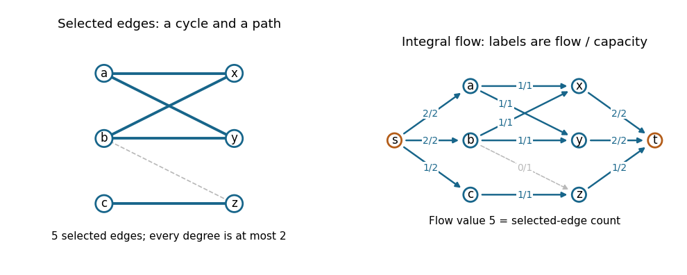
The blue edges in this example form a four-cycle in a graph and a one-edge graph path; the dashed edge is unused. Their five units of flow are optimal: the two left vertices $a,b$ can each contribute at most two selected edges, and $c$ has only one incident edge.

The constructed flow network has $|V|+2$ vertices and $|E|+|V|$ arcs. A polynomial-time algorithm for maximum flow, such as the Edmonds–Karp algorithm, followed by a traversal of the selected subgraph, gives an efficient solution.

The optimum radius is a distance from some city to a selected city, so it belongs toSort the distinct values of $D$, try them in increasing order, and run part (i)'s greedy procedure with each trial value $r$. Declare a trial successful when all cities are covered using at most $k$ centers; stop a failed trial as soon as a $(k+1)$st center would be selected. The trial $r=r^{\ast }$ must succeed by part (i), so the first successful value $\hat{r}$ satisfies $\hat{r}\le r^{\ast }$. Its output hasThere are $O(n^2)$ candidate distances and $O(n^2)$ work per trial, giving a polynomial-time algorithm with running time $O(n^4)$, plus sorting. Success at $r$ need not mean that radius $r$ itself is feasible; only the radius-$2r$ guarantee is used.

A faster alternative is the farthest-first traversal. Choose any first center, then repeatedly choose a city farthest from its nearest current center until $k$ have been chosen. Let $R$ be the resulting radius. If $R>0$, adjoin a city attaining that distance. At every earlier selection, the maximum distance to the then-current center set was at least $R$, so all pairs among these $k+1$ cities are at distance at least $R$. Two belong to the same optimal radius-$r^{\ast }$ closed ball, giving $R\le 2r^{\ast }$ by the triangle inequality. If $R=0$, the guarantee is immediate. Maintaining nearest-center distances gives $O(nk)$ distance evaluations without knowing $r^{\ast }$.

Use minimum-weight edge cover by matching savings. Reject inputs with an isolated vertex. For every vertex $v$, choose a cheapest incident edge $e_v$ and write $c_v=w(e_v)$. Define a baseline and a saving for each edge $uv$ byCompute a maximum-weight matching $M$ using $p$ as its weights, allowing the empty matching in a graph and imposing no maximum-cardinality condition. Negative savings may be ignored. ReturnThis is an edge cover. Since original weights are nonnegative, removing duplicate appearances of an edge cannot increase the total, and henceTo prove optimality, take a minimum-weight edge cover and remove redundant edges until it is inclusion-minimal. Nonnegative weights ensure that its weight does not increase, so it remains optimal. As proved in (i), its components are star graphs. Choose one edge from each star graph, forming a matching in a graph $N$.

In a star graph with center $a$, selected leaf $b$, and other leaves $L$, this choice contributes $w(ab)+{\sum }_{v\in L}{c}_v$ to $B-p(N)$. Each other leaf $v$ has its edge $av$ available, so $c_v\le w(av)$. Thus this contribution is at most the weight of that star graph. Summing over components yieldsSince $M$ maximizes saving, $p(M)\ge p(N)$, and consequentlyAll inequalities are equalities. Therefore $F_M$ is a minimum-weight edge cover. This proof also handles zero weights and duplicate cheapest-edge choices.

Finding all $c_v$ and constructing $F_M$ takes $O(|V|+|E|)$ time. A general-graph maximum-weight matching polynomial-time algorithm supplies the only substantial step; the documented routine runs in $O(|V{|}^3)$ arithmetic time. Exact rational or integer weights avoid floating-point comparisons affecting optimality.^[ref]

First test for an isolated vertex, reporting infeasibility if one exists. Otherwise compute a maximum cardinality matching $M$ using a general-graph polynomial-time algorithm, then add one arbitrary incident edge for each unmatched vertex in a matching. The proof in (i) shows that the resulting edge cover has minimum cardinality $|V|-|M|$.

The final scan takes $O(|V|+|E|)$ time with adjacency lists; the maximum cardinality matching computation is polynomial. One may obtain it from a general-graph maximum-weight matching routine with every weight equal to one.^[ref]

For the metric travelling salesman problem, a tour is a polynomial-size complexity certificate: list the vertices in cyclic visiting order. In polynomial time verify that every vertex occurs exactly once, add the encoded integer edge costs and compare the sum with the threshold. The certificate has $O(n\log n)$ bits, and addition uses a number of bits polynomial in the input length. If validity of the metric input is not treated as a promise, nonnegativity, symmetry and all triangle inequalities can also be checked in polynomial time. Therefore the decision problem belongs to NP.

An evaluation algorithm immediately decides a threshold instance by computing the optimum and comparing it with $L$. Conversely, suppose there is a polynomial-time decision algorithm. The optimum is an integer in $[0,nM]$, where $M$ is the largest edge cost; any fixed cyclic ordering gives the upper bound. Binary search on this interval using threshold queries finds the exact minimum. It makes $O(\log (nM+1))$ queries, and every queried threshold has polynomial encoding length. Thus the time is polynomial in the bit length, even when $M$ is numerically large. Zero-cost and trivial small instances can be handled directly. ConsequentlyThis concerns the optimum value; constructing an optimal tour is the separate optimization task.

For the hardness reduction, start with an undirected graph $G$ on $n\ge 3$ vertices and form the complete graph with costsThese costs satisfy the triangle inequality, since every direct cost is at most two and every two-edge path costs at least two. Set the threshold to $n$. Every tour has exactly $n$ edges, each costing at least one. Hence it has cost at most $n$ precisely when all its edges came from $G$, which is precisely the existence of a Hamiltonian cycle in $G$. The construction and threshold encoding are polynomial-time. Thus the assumed NP-completeness of the Hamiltonian circuit problem gives NP-hardness of metric TSP; together with its NP membership this proves NP-completeness of metric TSP decision.

For the approximation, compute a minimum spanning tree $T$. Deleting any one edge of an optimal tour leaves a spanning tree, so nonnegative costs implyDouble every tree edge. The resulting connected multigraph has even degrees and hence an Euler circuit, of cost $2c(T)$. Traverse it and skip previously visited vertices, except for the final return to the start. Each skip replaces a path by its direct edge; repeated use of the triangle inequality shows that no replacement increases cost. The result is a tour visiting every vertex exactly once and satisfyingThe Euler traversal and shortcutting take polynomial time, so the assumed polynomial-time MST routine supplies the requested polynomial-time algorithm. This is the double-tree approximation for metric TSP. In the relative-error convention, $c/\mathrm{OPT}-1\le 1$ when the optimum is positive, explaining the printed term “1-approximation”; in the multiplicative convention it is a factor-two approximation. If the optimum is zero, the same bound forces the returned tour to have zero cost as well.

Introduce slack variables $s_1,s_2,s_3$. The initial simplex dictionary isAll six variables are nonnegative. The given rule is the Dantzig pivot rule: select the nonbasic variable with the largest positive reduced cost. It applies to slack variables too once they become nonbasic. At each step the simplex ratio test limits how far that entering variable can increase before a basic variable reaches zero.

The successive objective rows of the simplex dictionary, expressed in the current nonbasic variables, areThese rows identify each entering variable unambiguously. Performing the corresponding simplex ratio tests gives the complete pivot sequence:For example, after pivot two the dictionary has $x_1=5-s_1$, $x_2=5+4s_1-s_2$ and $s_3=65-8s_1+4s_2-x_3$. Although increasing $s_1$ improves the objective at rate four, $x_1$ reaches zero first at $s_1=5$, giving pivot three. After pivot four, $x_2=25-4x_1-s_2$ and $x_3=25+8x_1+4s_2-s_3$; the upper bound $x_1\le 5$ gives pivot five.

In the final objective row every reduced cost is nonpositive. Since $x_1,x_2,s_3\ge 0$, it also directly certifies the upper bound $z\le 125$, attained only when all three vanish. Thus

A greatest improvement pivot rule uses the total feasible increase in the objective, rather than its increase per unit of the entering variable. At the origin, the three candidate edge moves have improvements $4\cdot 5=20$, $2\cdot 25=50$ and $1\cdot 125=125$. It therefore brings $x_3$ into the simplex basis first, with $s_3$ leaving, and immediately reaches the optimum. This rule solves this instance in one pivot.

This is a three-dimensional Klee-Minty cube example: the specified Dantzig pivot rule visits every vertex before reaching the optimum. Higher-dimensional versions require $2^d-1$ pivots, so that rule has exponential worst-case running time despite its strong practical performance. Each pivot requires only polynomially many arithmetic operations. An anti-cycling rule such as the Bland pivoting rule ensures finite termination; without one, degenerate pivots can cycle. A crude terminating bound is the number of possible bases, $\left(\genfrac{}{}{0ex}{}{m+n}{m}\right)$ for $m$ constraints and $n$ original variables, which can be exponential. This does not show that every conceivable pivot rule must take exponential time. Linear programming itself has polynomial-time algorithms, including the ellipsoid method and suitable interior-point methods.

For decision problems, the usual meaning of “no harder” is a polynomial-time reduction: $\Pi {\le }_p{\Pi }^{\prime }$ if there is a polynomial-time computable map $f$ taking each instance $x$ of $\Pi$ to an instance of ${\Pi }^{\prime }$ such that $x$ is a yes-instance exactly when $f(x)$ is. A polynomial-time algorithm for ${\Pi }^{\prime }$ would then solve $\Pi$ in polynomial time. A problem is NP-hard if every problem in NP admits such a reduction to it.

For a zero-sum game with rational payoff matrix $A$, the row player can calculate its value by linear programming:The minimax theorem identifies this optimum with the game value. Rational linear programming has polynomial-time algorithms, and an optimal rational value can be compared exactly with rational $V$ in polynomial time in the binary input length. Thus the decision problem belongs to P. If it were NP-hard, composing the reductions with this algorithm would put every problem in NP in P, contradicting the assumed separation. ThereforeThe finite rational encoding is part of the computational model; arbitrary real inputs without an encoding would not define the same complexity question.

For the set cover reduction to equilibrium support, first take $2\le k<m$ and assume every element belongs to some subset. Suppose rows $i_1,\dots ,i_k$ cover $S$. Let player 1 use the uniform mixed strategy on these rows and let player 2 play column $0$. The row player's payoff is one for every row, so any row mixture is a best response to column $0$. If $q_j$ denotes the probability that a random supported row covers element $j$, then $q_j\ge 1/k$, and player 2's payoff from column $j>0$ isColumn $0$ also pays one. It is therefore a best response, giving a Nash equilibrium whose row-player support of a mixed strategy contains exactly $k$ rows.

Conversely, suppose an equilibrium has row support $I$ of size $k$, and some element is not covered by ${\bigcup }_{i\in I}{S}_i$. For that column $q_j=0$, so player 2 can earn $k/(k-1)>1$. This is the largest possible column payoff, and it is attained exactly at columns corresponding to elements uncovered by $I$. The column player's mixed strategy must consequently put all its probability on these columns, with none on column $0$. Every currently supported row gives player 1 payoff zero. Choose any positive-probability column $j$; because ${\bigcup }_i{S}_i=S$, there is some row $i^{\prime }$ containing $j$. Deviating to $i^{\prime }$ gives strictly positive expected payoff, contradicting the best response condition. Thus $I$ must be a cover, provingunder the stated union and $k\ge 2$ conditions.

The printed formulation omits both conditions. For $k=1$, its payoffs contain division by zero. Without the union condition its claimed implication is false: take $n=2$, $m=3$, $k=2$ and $S_1=S_2=S_3=\{1\}$. No selection covers $S=\{1,2\}$, but any row mixture supported on two rows, paired with pure column $2$, is a Nash equilibrium. The row player always gets zero, and column $2$ is the column player's strictly optimal choice with payoff two. This gives an explicit counterexample to the unrestricted wording.

These restrictions do not weaken the complexity conclusion. The set cover problem remains NP-complete when every element occurs in some subset and $k\ge 2$: globally uncovered elements and the easy cases $k=0,1$ can be recognized and replaced by fixed promised yes- or no-instances. A cover by at most $k<m$ subsets can be padded to exactly $k$. The constructed game has polynomial size, so deciding whether a Nash equilibrium of the specified support size exists is NP-hard. Computing a complete description of all equilibria would resolve this question and hence is at least this difficult. In addition, the equilibrium set may be infinite; a complete output must then describe families rather than list individual points. There is a finite representation by feasible pairs of supports and their associated strategy polytopes, but there are exponentially many support pairs to consider. This reduction concerns locating specified supports or describing all equilibria, rather than finding one unrestricted equilibrium.

A decision problem belongs to NP if every yes-instance has a polynomial-length certificate verifiable by a deterministic polynomial-time algorithm. It is NP-hard if every problem in NP has a polynomial-time many-one reduction to it. It is NP-complete if it is both NP-hard and in NP.

A polynomial-time algorithm for any NP-complete problem would therefore give one for every problem in NP, implying $\mathrm{P}=\mathrm{NP}$. Conversely, if $\mathrm{P}=\mathrm{NP}$, all NP-complete decision problems have polynomial-time algorithms. NP-completeness does not unconditionally prove that polynomial-time solution is impossible. Optimization problems such as minimum tour cost are described as NP-hard, while their threshold decision versions can be NP-complete.

For a minimization problem with nonnegative costs, an approximation algorithm of ratio $\alpha \ge 1$ is a polynomial-time algorithm returning a feasible solution of cost at most $\alpha$ times the optimum on every instance. For maximization, one often uses $\alpha \ge 1$ with value at least $\mathrm{OPT}/\alpha$; an equivalent convention uses ratios at most one. The metric-tour question uses the minimization convention.

Let the bipartite graph have parts $L,R$. Add a source $s$, a sink $t$, capacity-one edges $s\to u$ for $u\in L$ and $v\to t$ for $v\in R$, and capacity $M=|V|+1$ on each original edge directed $L\to R$. Use the max-flow min-cut theorem: maximum flow value equals minimum cut capacity. Also use Integrality of the Ford-Fulkerson algorithm: integral capacities admit an integral maximum flow, found by integral augmenting paths.

An integral flow selects a matching in a graph, because each left and right vertex carries at most one unit. Conversely every matching gives a unit flow along its selected $s\to u\to v\to t$ paths. Hence maximum flow value equals maximum matching cardinality.

A minimum cut has capacity at most $|L|$, whereas crossing even one original edge would cost $M>|L|$. For its source side $Z$, no edge of the original graph runs from $L\cap Z$ to $R\setminus Z$. Thereforeis a vertex cover, and its cardinality is exactly the cut capacity. Conversely, given any cover $U$, use $Z=\{s\}\cup (L\setminus U)\cup (R\cap U)$. No original edge crosses this cut, because both its endpoints would otherwise be outside the cover; its capacity is $|U|$. Thus minimum cut capacity equals minimum cover size, proving Kőnig's theorem for bipartite matching:For the algorithm, repeatedly find augmenting paths in the residual network, then take $Z$ to be the vertices reachable from $s$. Each integral augmentation increases flow by at least one; the total value is at most $\min (|L|,|R|)$. Each reachability search takes $O(|V|+|E|)$ time, so this procedure takes $O(|V|(|V|+|E|))$ time. The network uses only polynomially many edges and integer capacities, yielding the requested polynomial-time algorithm and an explicit cover.

Automated planning with ground actions that are always applicable because their precondition sets are empty. Delete effects are still permitted, so taking the union of all add effects does not decide reachability. With a positive conjunctive goal, the last-achiever algorithm for precondition-free planning gives a polynomial-time algorithm.

Let $P$ be a nonzero multivariate polynomial over a field $K$, with total degree at most $d\ge 0$. Choose a nonempty finite set $S\subseteq K$. For independent random variables $a_1,\dots ,a_n$, each with a uniform distribution on a finite set on $S$, the Schwartz-Zippel lemma givesNonzeroness is essential; the zero polynomial always evaluates to zero. The total degree sums exponents within each monomial, rather than taking their maximum: $x^2{y}^3+y$ has total degree five. The field need not be finite, but $S$ must be finite. The estimate reduces error only when $d/|S|<1$.^[ref]

The proof begins with the root bound for a polynomial. For several variables, write $P={\sum }_{j=0}^m{Q}_j(x_1,\dots ,x_{n-1})x_n^j$, with $Q_m\ne 0$. The total degree of $Q_m$ is at most $d-m$. By induction, $Q_m$ vanishes with probability at most $(d-m)/|S|$. Otherwise the remaining univariate polynomial has at most $m$ polynomial roots. Adding the two contributions gives $d/|S|$.^[ref]

The algorithm samples a point, performs exact polynomial evaluation, rejects the identity if the value is nonzero, and otherwise accepts. The lemma bounds false acceptance for every fixed nonzero input. For the polynomial identity testing over a finite field example, $G$ has $d=2$ and $|S|=5$, so its exact $2/5$ error attains the bound. Numerical near-zero values from floating-point arithmetic do not satisfy this exact algebraic contract. A polynomial-time algorithm claim additionally needs efficient sampling and evaluation, including the bit cost of representing and operating on field elements. Counting field operations alone does not establish that cost.