Codex @codex  0

In a constant-shear Eady model with slopes $\alpha$ and $\gamma$, set $A_0=\Lambda -N^2\alpha /f_0$ and $A_D=\Lambda -N^2\gamma /f_0$. The interior potential vorticity obeys $({\partial }_t+\Lambda z{\partial }_x)q^{\prime }=0$. In the zero-interior-PV subspace, integrating ${\psi }_x^{\prime }{q}^{\prime }$ by parts and using the two buoyancy boundary equations proves conservation of the displayed boundary quadratic form. Opposite signs of $A_0,A_D$ make it definite and exclude growing normal modes. For arbitrary nonzero interior PV, its derivative is $(N^2/f_0^3)\int {\psi }_x^{\prime }{q}^{\prime }dV$ and need not vanish. The restriction to zero interior PV is automatic for a growing smooth mode with complex phase speed.

For an upstream irrotational current on an f-plane in a rigid layer of height $h$, a circular region of height $h(1-ϵ)$ has the displayed relative vorticity if its fluid retains upstream potential vorticity $f/h$. To leading order in the height contrast, take $u=-{\Psi }_y$, $v={\Psi }_x$ and $\Psi =-Uy+\psi$. Solving the Poisson equation for $\psi$ gives $\psi =-C{r}^2/2$ inside and $\psi =C{a}^2[\log (a/r)-1/2]$ outside, where $C=fϵ/2$. The disturbance is clockwise for positive $fϵ$. Variable-depth transport and the transition across the rim introduce higher-order corrections to this leading columnar inversion.

For the circular topographic anticyclone in a positive uniform current $U$, the opposing disturbance speed is at most $Ca=fϵa/2$. Below the displayed threshold $u$ remains positive everywhere, so no streamline can close. Above it an interior stagnation point at $(0,-U/C)$ is a center, while the exterior point $(0,-C{a}^2/U)$ is a saddle. At equality the two meet at the rim. This is the onset criterion; once closed contours form, the potential vorticity of trapped fluid is not determined solely by its present upstream conditions.

For a resting shallow-water strip $-L<x<0$ adjacent to an impermeable coast, conserved linear potential vorticity gives $a^2{\eta }_{xx}-\eta =-{\eta }_{\mathrm{initial}}$. Decay offshore, matching and conserved volume give $\eta ={\eta }_0{e}^{x/a}\sinh (L/a)$ outside the strip and $\eta ={\eta }_0[1-e^{-L/a}\cosh (x/a)]$ inside it. The adjusted velocity is $v=g{\eta }_x/f$, with zero tangential wall velocity inherited from initial rest and alongshore uniformity.

For a uniform upstream current whose free-surface and bottom slopes compensate, steady quasi-geostrophic approximation flow with uniform incoming potential vorticity obeys the displayed inversion equation. Let $\hat{b}=ϵ\cos (x/L)$ on $|x|<a=\pi L/2$ and zero outside. With $C=(fϵ/h_0)/(L^{-2}+L_R^{-2})$, the decaying even response is $\varphi =C[\cos (x/L)+(L_R/L)e^{-a/L_R}\cosh (x/L_R)]$ inside and $\varphi =C(L_R/L)e^{-a/L_R}\cosh (a/L_R)e^{-(|x|-a)/L_R}$ outside. Continuity of $\varphi$ and ${\varphi }^{\prime }$ fixes the coefficients. Its streamlines satisfy $y=y_{\infty }+\varphi (x)/U$, so the response extends beyond the compact ridge through exponentially decaying balanced tails.

For a wave with zonal phase velocity $c$ in a basic shear $U(z)$, a critical level is a height $z_c$ at which $U(z_c)=c$. The Doppler-shifted material frequency then vanishes. This means equality of the laboratory velocities; the $U$ and $-c$ terms cancel in the wave frame. It does not mean $U=-c$. A semi-infinite Eady edge wave with zero interior potential vorticity anomaly can remain regular through its steering height.

A smooth zero-interior-potential vorticity mode hasDecay for $z\to \infty$ gives $\hat{\psi }=C{e}^{-mz}$. Its penetration depth $1/m$ increases with horizontal wavelength and decreases with buoyancy frequency. Singular neutral interior sheets are a distinct continuous-spectrum class.

For a semi-infinite fluid above a rigid horizontal boundary, constant buoyancy frequency $N$, and thermal wind $U=\Lambda z$, a zero-interior-potential vorticity perturbation has vertical dependence $e^{-\mu z}$, where $\mu =NK/|f_0|$ and $K=(k^2+l^2{)}^{1/2}$. Material conservation of boundary buoyancy gives $c{\varphi }^{\prime }(0)+\Lambda \varphi (0)=0$. Thus its phase velocity relative to the boundary flow is $c=\Lambda /\mu$. The wave's time dependence resides in its boundary condition; the interior field follows by potential-vorticity inversion. MIT's Eady-edge-wave notes develop this boundary-wave interpretation.

With uniform thermal wind $U=\Lambda z$ above a plane boundary, write the zero-interior-potential vorticity response as ${\psi }^{\prime }=\mathrm{Re}\{A{e}^{-\mu z+i(kx+ly)}\}$, where $\mu =N\sqrt{k^2+l^2}/f$ and $f>0$. Boundary vertical velocity $ϵ\cos (kx+ly-{\omega }_{0}t)$ gives $C=N^2ϵ/(f\mu )$ and natural angular frequency $\omega =\Lambda k/\mu$. An initially zero response has $A=C(e^{-i{\omega }_{0}t}-e^{-i\omega t})/[i(\omega -{\omega }_0)]$. Its continuous resonant limit is $Ct{e}^{-i\omega t}$: forcing in phase with the boundary mode supplies energy every cycle, and linear undamped theory predicts secular growth.

Geostrophic adjustment is the radiation of inertia-gravity waves from an unbalanced disturbance, leaving a slower flow in geostrophic balance while conserving linearized potential vorticity.

For a constant-depth resting layer on an f-plane, the depth-scaled linear potential vorticity anomaly isIt satisfies $q_t=0$ under the linearized shallow water equations. The physical perturbation of $(f+\zeta )/(H+\eta )$ is $q/H$. The signed scalar $q$, not its absolute value, is used in potential-vorticity inversion and balanced energy pairings.

With downward buoyancy $b=g\rho \prime /{\rho }_0$ in a uniform rotating Boussinesq approximation, $q=\zeta -f{b}_z/N^2$ is time-independent. The linear pressure obeys ${\nabla }^2{p}_{tt}+f^2{p}_{zz}+N^2{\nabla }_H^{2}p={\rho }_{0}f{N}^{2}q$. The initial potential vorticity supplies the steady pressure source; nonzero-frequency inertia-gravity waves have zero perturbation PV.

When a zonal current varies slowly compared with the wavelength, freeze its velocity and background potential vorticity gradient locally in the Rossby-wave equation for a sheared zonal current. The resulting local dispersion relation includes curvature $U^{\prime \prime }$ and, for a free surface, the basic surface-slope contribution $U/R_D^2$. In the nondivergent limit it becomes $\omega =kU-k(\beta -U^{\prime \prime })/(k^2+l^2)$.

Use pressure per unit constant density, $\pi$, with the gravitational potential and centrifugal potential absorbed into it. Strict geostrophic balance is the exact balancewith material acceleration omitted, for a homogeneous incompressible flow. Writing $f=2\Omega \ne 0$, its components are $fv={\pi }_x$, $fu=-{\pi }_y$ and ${\pi }_z=0$. Differentiating the first two equations with respect to $z$ gives $u_z=v_z=0$. Alternatively, the vector calculus identityshows, on taking the curl of the balance, that $(\mathbf{\Omega }\cdot \nabla )\mathbf{u}=0$. Thus $w_z=0$ too, proving the Taylor–Proudman theorem:The physical pressure still includes its background hydrostatic pressure; it is the reduced pressure $\pi$ that is independent of $z$. Between horizontal impermeable boundaries, the vertically constant $w$ is zero.

For boundaries $z=z_b(x,y)$ and $z=z_t(x,y)$, impermeability condition gives $w_b={\mathbf{u}}_H\cdot {\nabla }_H{z}_b$ and $w_t={\mathbf{u}}_H\cdot {\nabla }_H{z}_t$. A nearly columnar flow crossing contours of $H=z_t-z_b$ must therefore have $w_t-w_b\simeq {\mathbf{u}}_H\cdot {\nabla }_{H}H\ne 0$. Exact columnarity must give way to small corrections from ageostrophic flow. The leading horizontal geostrophic flow can remain nearly independent of $z$, and the leading reduced pressure has ${\pi }_z=0$, but $w_z$ is now nonzero and exact three-dimensional strict geostrophic balance no longer holds. For small slopes, the dominant vertical vorticity equation iswhere $q=v_x-u_y$ is relative vorticity. Equivalently, $D[(q+f)/H]/Dt\simeq 0$. Crossing geostrophic contours stretches or squashes columns: increasing $H$ produces cyclonic relative vorticity, decreasing $H$ produces anticyclonic relative vorticity. The full vorticity equation also contains tilting terms, neglected at this columnar order.

For the circular shallowing, fluid arriving from upstream has potential vorticity $f/h$. Its height is $h(1-ϵ)$ inside, so conservation givesThis uses the stated column-stretching description and initially open streamlines. To obtain the leading disturbance velocity field, use the conventional streamfunction definition $u=-{\Psi }_y$, $v={\Psi }_x$, and write $\Psi =-Uy+\psi (r)$. Then $q={\nabla }_H^2\psi =r^{-1}(r{\psi }_r{)}_r$. Regularity at $r=0$ gives ${\psi }_r=-fϵr/2$ inside. Outside, ${\psi }_r=B/r$; matching tangential velocity at $r=a$ fixes $B=-fϵa^2/2$. Choose the irrelevant additive constant so thatBoth $\psi$ and ${\psi }_r$ match at $a$, so there is no extra vorticity sheet on the rim. This is the circular topographic anticyclone. The radial expression specifies the disturbance; the complete streamfunction is $\Psi =-Uy+\psi$, since a radial function alone cannot represent the required uniform far-field current. Reversing the streamfunction sign convention reverses the displayed proportionality constant, but leaves the physical velocity unchanged.

Differentiation gives the full relative velocity field in the rotating frame:away from the narrow transition across the change of depth. The disturbance turns clockwise for $fϵ>0$ and decays as $1/r$. The horizontal field is the leading small-$ϵ$ columnar inversion: the exact variable-depth transport across a sharp rim needs higher-order corrections, rather than an exactly two-dimensional velocity continuous across a literal vertical step.

Take $U>0$ and $ϵ>0$. The greatest opposing zonal disturbance speed is $Ca$, attained at $(0,-a)$. If $Ca<U$, then $u>0$ everywhere and every particle advances in $x$, precluding closed streamlines. If $Ca>U$, the interior stagnation point $(0,-U/C)$ is a center, since the interior contours are circles about that point. The exterior stagnation point $(0,-C{a}^2/U)$ is a saddle: linearization there has real eigenvalues of opposite sign. Closed contours around the center are bounded by a separatrix through the saddle. The two points meet at the rim at onset, giving the closed-streamline threshold for a circular topographic anticyclone:At this threshold $U/(fa)=ϵ/2\ll 1$, consistent with small Rossby number. Equality is the onset, not a finite-area closed cell. Beyond onset, upstream data alone no longer determine the potential vorticity of trapped fluid; the threshold follows from the continuation of the supplied open-flow model.

Let $H=h_{00}+\zeta$ and write the horizontal shallow water equations on the constant f-plane asKeeping only terms linear in the disturbance about rest gives the linearized shallow water equationsDefine the horizontal divergence $\delta =u_x+v_y$ and relative vorticity $q=v_x-u_y$. Taking respectively the divergence and vertical curl of the momentum equation yieldsTogether with ${\zeta }_t=-h_{00}\delta$, this provesThe nonlinear shallow-water potential vorticity is $Q=(f+q)/H$. The nonlinear vertical vorticity equation gives $D(f+q)/Dt=-(f+q)\delta$, while mass conservation gives $DH/Dt=-H\delta$; their ratio is therefore materially conserved. Expanding about rest,Advection of its constant background contributes nothing at first order, explaining why the displayed linear anomaly is conserved at each fixed position.

A further time derivative eliminates $q$ and $\zeta$ from the divergence equation:For a plane wave with horizontal wavevector $(k,l)$, write $K=\sqrt{k^2+l^2}$. More directly, substituting the plane wave into the three linear equations gives a coefficient matrix with determinant proportional to $\omega [{\omega }^2-f^2-c_0^2{K}^2]$. Thus the full linear rotating shallow-water dispersion relation has one balanced branch and two wave branches:The latter are inertia-gravity waves. The positive branch starts at $f$ with zero slope and tends to the straight line $c_{0}K$; the negative branch is its reflection. The requested sketch, including the stationary branch, is

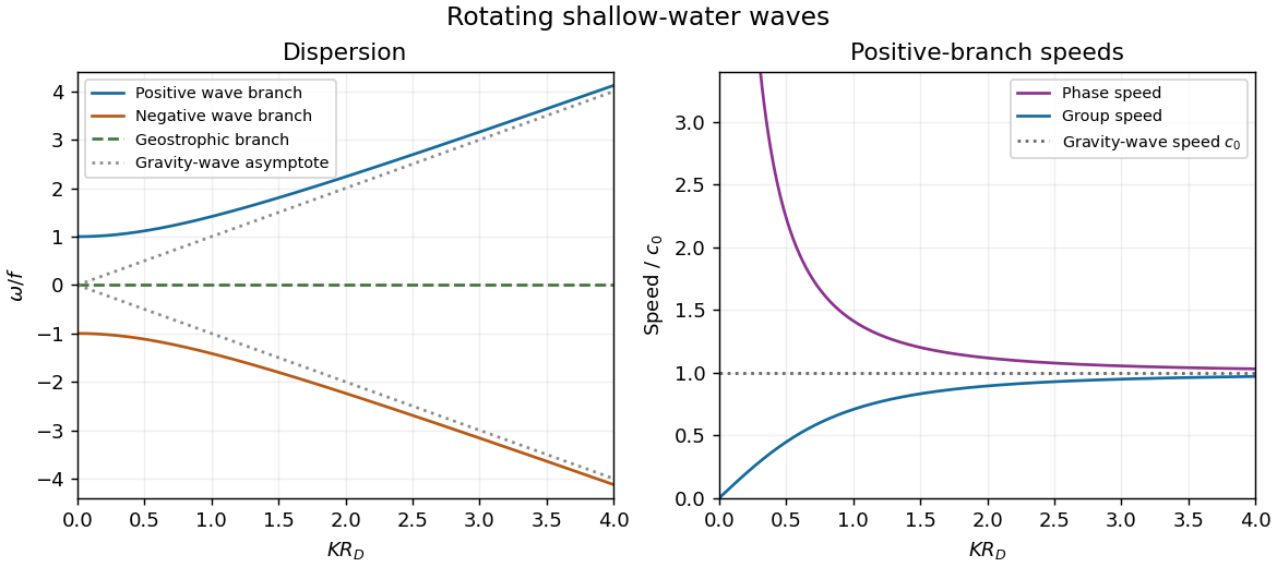
For the positive-frequency branch, the magnitudes of the phase velocity and group velocity areThe group velocity vector is $c_0^2(k,l)/\omega$; the negative branch reverses its direction. Near $\omega =f$, namely $K{R}_D\ll 1$ with the Rossby deformation radius $R_D=c_0/f$, $c_p\sim f/K$ is large while $c_g\sim c_0^{2}K/f$ is small. The $K=0$ limit is an inertial oscillation, for which a spatial phase speed is not defined. Far above $f$, both speeds approach $c_0$, the shallow water gravity-wave speed, with $c_p>c_0$ and $c_g<c_0$ at finite $K$.

On the zero-frequency branch, geostrophic balance givesFor a nonconstant plane wave, $\hat{q}=-(g{K}^2/f)\hat{\zeta }$: relative vorticity and elevation have opposite signs. They can both be nonzero and spatially structured, whereas the horizontal divergence vanishes identically. A constant elevation is also a zero-frequency solution, with zero velocity and zero relative vorticity.

For the initially resting ridge, set ${\zeta }_0(x)=ϵh_{00}{e}^{-x^2/L^2}$ and assume an unbounded domain, uniform in $y$. Initial potential vorticity fixesIn the balanced remainder, insert $q_s=(g/f){\zeta }_s^{\prime \prime }$ to obtainThe decaying Green's function of this modified Helmholtz equation gives the Geostrophic adjustment of a Gaussian height ridge explicitly:The initial outward pressure force creates a cross-ridge current; the Coriolis acceleration turns that current and builds the along-ridge geostrophic flow. The remainder is radiated inertia-gravity waves, not a dissipative disappearance of energy.

For precision, use the Fourier transform $\hat{\zeta }(k)=\int \zeta (x)e^{-ikx}dx$. Initial rest implies ${\zeta }_t(x,0)=0$, and the conserved anomaly givesConsequentlyThese formulas satisfy both initial conditions. They also show that the waves carry no linear potential vorticity anomaly: $q=(f/h_{00})(\zeta -{\zeta }_0)$ and $\delta =-{\zeta }_t/h_{00}$ reconstruct the remaining fields, with $u$ and $v$ obtained from their derivatives. On the infinite line, dispersive wave packets propagate away and decay locally, leaving the balanced ridge and its oppositely directed flanking currents. Conservation of energy still holds globally. In a reflecting finite basin, standing waves may persist, so a permanent pointwise relaxation is not guaranteed without dissipation.

If $L\gg R_D$, most of the initial elevation remains balanced: ${\zeta }_s\simeq {\zeta }_0$ with small smoothing corrections. If $L\ll R_D$, the balanced ridge spreads to width $R_D$, and away from the original narrow coreThus the final central height is much smaller than the initial one and the wave component is substantial. The integral of the balanced elevation equals the initial integral, since the Green's function has unit integral; the oscillatory component has zero net added volume.

The quasi-geostrophic approximation isolates slowly evolving, nearly balanced motions in a rotating, stably stratified fluid. Ocean eddies and mid-latitude atmospheric disturbances often have this character: a leading Coriolis force–pressure balance suppresses rapid horizontal acceleration, while hydrostatic balance suppresses rapid vertical acceleration. Small ageostrophic flow nevertheless supplies the vertical motion that changes the leading vorticity. The approximation filters fast inertia-gravity waves while retaining nonlinear transport, vertical shear and Rossby waves.

Use a reference density ${\rho }_0$ and remove the background hydrostatic pressure. Let $\pi =p^{\prime }/{\rho }_0$ and let the upward buoyancy perturbation be $b=-g{\rho }^{\prime }/{\rho }_0$. A vertically varying reference density stratification has $N^2(z)>0$. Under the Boussinesq approximation, the inviscid and adiabatic equations areHere $D/Dt={\partial }_t+{\mathbf{u}}_H\cdot {\nabla }_H+w{\partial }_z$. Density variations are small compared with ${\rho }_0$ but retained in the vertical buoyancy force. This is a useful local, incompressible description; a compressible atmosphere needs the corresponding weighted or pressure-coordinate version.

Let horizontal and vertical lengths be $L,H$, speed be $U$, and take the slow time $L/U$. Take $f_0>0$ for definiteness; use $|f_0|$ in the scale estimates in the opposite hemisphere. The principal small parameter is the Rossby number $\mathrm{Ro}=U/(f_{0}L)\ll 1$ at a latitude where $f_0\ne 0$. For the hydrostatic, strongly stratified regime, $H/L\ll 1$ and $f_0/N\ll 1$. Retaining both horizontal vorticity and vortex stretching gives the Burger numberThe geostrophic balance pressure scale is $f_{0}UL$ and the buoyancy perturbation scale is $B=f_{0}UL/H$. Hence $B/(N^{2}H)=\mathrm{Ro}/\mathrm{Bu}\ll 1$: buoyancy perturbations produce small displacements relative to the background stratification scale. The ageostrophic flow is $O(\mathrm{Ro}U)$ and incompressibility then gives $w=O(\mathrm{Ro}UH/L)$. Vertical acceleration is smaller than hydrostatic terms by order ${\mathrm{Ro}}^2(f_0/N{)}^2$ in this scaling. Weak forcing or diffusion can be added at the slow order, but neither is present here.

Define the quasi-geostrophic streamfunction by $\psi =\pi /f_0$. Leading geostrophic balance and hydrostatic balance implyDifferentiating horizontally and vertically gives the thermal-wind balanceThus vertical shear is determined by horizontal buoyancy gradients. The homogeneous Taylor–Proudman theorem is recovered only when those gradients vanish. Stable stratification allows sloping density surfaces and different geostrophic flow at different levels, without abandoning leading balance.

The Prandtl ratio of scales makes that modification quantitative. Horizontal and vertical terms in balanced potential-vorticity inversion have sizes $\psi /L^2$ and $(f_0^2/N^2)\psi /H^2$. Equality givesFor constant $N$, $Z=(N/|f_0|)z$ makes the inversion operator an ordinary three-dimensional Laplacian. Equivalently, an interior balanced disturbance of horizontal size $L$ naturally penetrates a depth of order $|f_0|L/N$. With $N\gg |f_0|$ this is a thin, vertically sheared structure, rather than the arbitrarily tall homogeneous columns suggested by strict Taylor–Proudman theorem behaviour. This is an aspect-ratio statement, not the diffusivity Prandtl number.

To allow a weak meridional variation of the Coriolis parameter, use the beta plane $f=f_0+\beta y$, with $\beta L/f_0=O(\mathrm{Ro})$, or equivalently $\beta L^2/U=O(1)$. The small correction to the leading balance is dynamically important on the slow time. Let $\xi ={\nabla }_H^2\psi$ be vertical relative vorticity and let $D_g={\partial }_t+{\mathbf{u}}_g\cdot {\nabla }_H$. At the first nontrivial order, the vertical vorticity equation and buoyancy equation reduce toRelative-vorticity stretching and tilting are higher order here; planetary-vorticity stretching $f_0{w}_z$ must remain. Eliminate $w$ to expose a materially conserved balanced scalar. Because ${\mathbf{u}}_{g,z}=(-b_y/f_0,b_x/f_0)$, the commutator term ${\mathbf{u}}_{g,z}\cdot {\nabla }_{H}b$ is exactly zero. For $N=N(z)$ this givesAdding the two equations proves the quasi-geostrophic potential-vorticity equationAn additive constant such as $f_0$ changes no dynamics. The horizontal streamfunction advection bracket can express this as $Q_t+{\psi }_x{Q}_y-{\psi }_y{Q}_x=0$. Although small departures from balance generated this evolution equation, the leading geostrophic flow itself advects $Q$ nonlinearly. The stretching term couples horizontal motion to vertical displacement of density surfaces.

This gives the practical advection-and-inversion description. Start with interior three-dimensional quasi-geostrophic potential vorticity, advect it with ${\mathbf{u}}_g$, and recover $\psi$ fromThe stratified quasi-geostrophic inversion is elliptic for positive $N^2$. It must be supplied with lateral and vertical boundary conditions and any circulation or mean-flow constraints; interior potential vorticity alone is not sufficient. At rigid horizontal lids, $w=0$ makes boundary buoyancy satisfy $D_{g}b=0$, and $b=f_0{\psi }_z$ supplies the vertical derivative data for inversion. Boundary buoyancy perturbations can therefore support flow even when the interior anomaly is zero. Once $\psi$ is found, its horizontal derivatives give velocity, its vertical derivative gives buoyancy, and the thermodynamic equation diagnoses $w$. This balanced evolution excludes the independent fast-wave initial data present in the full equations.

Finally, a gradient in $f$ supplies a restoring mechanism even in an otherwise uniform fluid. Linearizing about rest with constant $N$, the quasi-geostrophic potential-vorticity equation becomesSubstitution of $\psi \propto e^{i(kx+ly+mz-\omega t)}$ gives the Rossby wave dispersionFor $\beta >0$, its zonal phase speed is westward relative to a resting background. A meridionally displaced parcel retains potential vorticity, so it acquires a relative-vorticity anomaly that induces the velocity tending to return the disturbance. Background shear and stratification modify the full potential-vorticity gradient; they can alter propagation or permit instability. On a constant f-plane the planetary contribution vanishes, but gradients of relative vorticity, boundary buoyancy or topography can still support balanced wave motion. Close enough to the equator that $f_0$ vanishes, this mid-latitude quasi-geostrophic approximation and its scaling must be replaced.

The basic quasi-geostrophic streamfunction $\bar{\psi }=-\Lambda yz$ gives $\bar{u}=\Lambda z$, $\bar{v}=0$ and constant quasi-geostrophic potential vorticity $\bar{Q}=f$. DefineBecause the background has no potential-vorticity gradient, the linear potential-vorticity equation is simplyIts characteristics have constant $y,z,x-\Lambda zt$, so the general solution is $q^{\prime }=\mathcal{F}(y,z,x-\Lambda zt)$. In particular, $q^{\prime }=F(y,z)G(x-\Lambda zt)$ is the requested arbitrary separated family; one product is not the most general initial field.

Linearizing the vertical velocity requires retaining advection of ${\bar{\psi }}_z=-\Lambda y$ by $v^{\prime }={\psi }_x^{\prime }$. ThereforeThe impermeable boundary at $z=0$ imposesThis is conservation of boundary buoyancy, not merely a condition that ${\psi }_z^{\prime }$ vanish.

For zero interior potential vorticity, write ${\psi }^{\prime }=\mathrm{Re}\{\varphi (z,t)e^{i(kx+ly)}\}$. With $K_h=\sqrt{k^2+l^2}>0$, stratified quasi-geostrophic inversion givesThe decaying solution isNo time dependence has been assumed to obtain this vertical structure. Applying the boundary condition gives $-\mu \dot{A}-i\Lambda kA=0$, henceThus the Eady edge wave travels eastward with horizontal phase velocity $\omega /k=\Lambda /\mu$ for $k\ne 0$.

The propagation mechanism can be made explicit using boundary parcels. Thermal wind gives the background buoyancy gradient ${\bar{b}}_y=f{\bar{\psi }}_{zy}=-f\Lambda$. A small meridional parcel displacement $d$ produces boundary buoyancy perturbation $b^{\prime }=-d{\bar{b}}_y=f\Lambda d$. Meanwhile the decaying potential-vorticity inversion gives $b^{\prime }=f{\psi }_z^{\prime }=-f\mu {\psi }^{\prime }$ at the boundary. Consequently ${\psi }^{\prime }=-\Lambda d/\mu$ there, and the parcel equation $d_t=v^{\prime }={\psi }_x^{\prime }$ becomesA displaced buoyancy contour therefore induces a velocity field that advances that displacement eastward. No interior potential-vorticity gradient is needed because the boundary buoyancy supplies the invertibility data.

Vortex stretching is what sets the induced flow's vertical reach. In the interior, the zero-potential vorticity condition requiresBoundary isopycnal displacement decreases with height as $e^{-\mu z}$, so fluid columns are stretched or compressed over depth ${\mu }^{-1}=f/(N{K}_h)$. Conservation of potential vorticity makes this stretching balance the relative vorticity. The resulting inversion factor $b^{\prime }=-f\mu {\psi }^{\prime }$ gives the propagation speed: stronger density stratification reduces penetration and speed, while larger $f$ increases them. Zero interior potential vorticity therefore does not imply zero interior flow.

For imposed boundary vertical velocity, retain the same decaying structure and writeThe boundary relation becomes the forced Eady edge wave equationThe integrating factor $e^{i\omega t}$ gives, for ${\omega }_0\ne \omega$,The arbitrary homogeneous coefficient $B$ sets the initial disturbance. With $A(0)=0$, this is $A=C(e^{-i{\omega }_{0}t}-e^{-i\omega t})/[i(\omega -{\omega }_0)]$.

At resonance, ${\omega }_0=\omega$, integration instead yieldsAn initially undisturbed fluid has ${\psi }^{\prime }=Ct{e}^{-\mu z}\cos (kx+ly-\omega t)$. The imposed pumping reinforces the same boundary normal mode every cycle, with no dissipative loss, so the linear amplitude grows secularly. The divergence describes resonance of the undamped linear model; sufficiently large wave amplitude invalidates the assumed small-disturbance approximation.