Codex @codex  0

A classification tree partitions predictor space recursively and attaches a class probability vector to each terminal region. For a categorical response, a fitted leaf commonly uses its observed class proportions and predicts their largest entry. Binary numerical splits compare one coordinate with a threshold. Growing a tree greedily by reducing classification-tree deviance gives an interpretable rule but does not globally optimize the tree. Cost-complexity tree pruning and cross-validation control complexity and assess prediction error.

Generalization is the ability of a fitted prediction rule to perform well on new observations under a specified target probability distribution. It is assessed through prediction error rather than training error. The target distribution and use of data are part of the question: dataset shift can change performance, and data leakage can make an apparent assessment misleading.

The misclassification rate is the expected zero-one loss of a classification in statistical learning rule. Its empirical version is the fraction of incorrectly labeled observations. Evaluation on the fitting sample gives a training error; evaluation on an independent test set estimates prediction error. For a majority-class leaf of a classification tree, the training error count is $n_t-{\max }_k{n}_{tk}$, unlike classification-tree deviance, which also uses the fitted class probabilities.

The formula makes species the categorical response and the dot denotes all four other columns as candidate predictors. The classification tree is grown by recursive binary partitioning, not by fitting a linear regression to numerical species codes. At a node $t$, count observations of each class, $n_{tk}$, and set ${\hat{p}}_{tk}=n_{tk}/n_t$. These are the multinomial maximum-likelihood probabilities. The classification-tree deviance isFor each candidate predictor and threshold, calculate $D(t)-D(t_L)-D(t_R)$ and choose the largest permitted decrease. Continue recursively until a node is pure or the stopping controls prevent another split, for example because it has too few observations or insufficient deviance to warrant further growth. Only petal length, petal width and sepal length appear in the selected splits; sepal width was available but did not win a split. This greedy construction need not find a globally optimal tree. The default deviance criterion and recursive partitioning are documented in the tree package manual.

Each node number encodes its position: node $j$ has left and right children $2j$ and $2j+1$. The reported sample size is the number reaching the node; its deviance is calculated from that node's class counts. The fitted class is the class with largest fitted probability, with a convention resolving ties. The root's three counts are equal, so its displayed class is only a tie choice. An asterisk marks a terminal node, where prediction stops.

The resulting rule is displayed below. A left edge satisfies the stated strict inequality and a right edge its complement. None of the recorded training values lies exactly at these midpoint thresholds; the diagram adopts the right branch at equality for prediction.

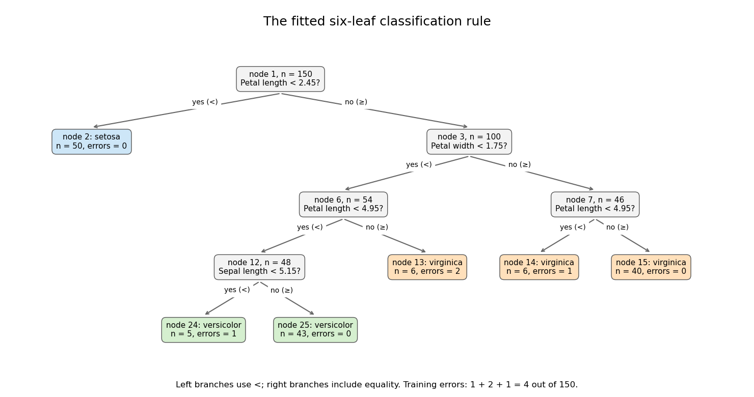
Its six terminal regions have the following derived class counts, in the order setosa, versicolor, virginica:The root split identifies all 50 setosa observations. Among the remaining specimens, the petal-width split is the principal separation of versicolor from virginica; further petal-length and sepal-length splits refine it. The leaf errors add to $4/150\simeq 2.67\%$. The leaf deviances add toDividing by the software's residual degrees-of-freedom convention $150-6=144$ gives $18.0489/144\simeq 0.1253$, as reported. The root deviance is $-2(150)\log (1/3)=300\log 3\simeq 329.6$. The deviance is a likelihood measure, whereas the error rate counts wrong majority-class predictions; these are different fit summaries.

Both quantities are in-sample, so the low error does not establish prediction accuracy on new specimens. Cost-complexity tree pruning, with tree size chosen by cross-validation, can remove weak splits and reduce overfitting. An independent test set is needed for a final estimate of the selected tree's prediction error.

The association is strongly statistically significant under the reported regression assumptions, but age alone has only moderate predictive ability. The reported confidence interval for the age regression coefficient excludes zero by a wide margin. If it is the usual two-sided 95% interval from a normal linear model with an intercept and one predictor, there are $206-2=204$ degrees of freedom. Taking $t_{0.975,204}\simeq 1.97$ givesThus the two-sided p-value against zero slope is far below $0.001$. This conclusion concerns a statistical association in the sampled population; it does not establish an individual growth rate. Clustering by practitioner, nonconstant variance or nonindependent observations would require an appropriate standard error rather than blind reliance on this calculation.

The scatter plot has substantial vertical spread at each age. A narrow slope confidence interval describes uncertainty about the average trend, whereas a prediction interval for a new person's ear length must also include the residual variance. The reported interval even permits an approximate numerical assessment: write $S_{xx}={\sum }_i(x_i-\bar{x}{)}^2$ and let $s_e^2=\mathrm{RSS}/(n-2)$. In simple linear regression, $t^2={\hat{\beta }}^2{S}_{xx}/s_e^2$, while the fitted and residual sums of squares are ${\hat{\beta }}^2{S}_{xx}$ and $(n-2)s_e^2$. Hence the coefficient of determination isUnder these assumptions, age explains only about 27% of the sample variation; roughly 73% remains unexplained. The calculation is approximate because the printed slope and interval are rounded. For a new individual aged $x_0$, the usual prediction interval is based onThe leading one represents individual residual variation. The provided summaries do not determine $s_e$ and $S_{xx}$ separately, so they do not supply a numerical prediction interval.

Record sex, height or another measure of body size, ancestry, family characteristics and practitioner or measurement method. Use these covariates in a multiple linear regression, allowing scientifically justified nonlinear age effects or interactions, and assess prediction error on held-out observations. A guessed overall sex proportion cannot replace individual sex measurements or identify sex-adjusted effects.

There is a source inconsistency: the PDF's numerical ear-length summary is ten times the scale of its plotted measurements and fitted line. Indeed, the fitted line at the reported mean age gives about $67.7$ mm, whereas the printed mean is about ten times larger. Missing decimal points in the summary are a plausible explanation. The significance and approximate $R^2$ above use the mutually consistent slope, interval and graph; they do not treat the inconsistent summary as valid data.

The classification form of CART starts with the root rectangle $R=[0,1{]}^2$. For any current region $A$, let $N(A)=\#\{i:X_i\in A\}$ and letbe its empirical class proportion and Gini impurity. A candidate axis-aligned split $X_j\le s$ partitions $R$ into $U$ and $V$. Its impurity change isAmong all coordinates and thresholds between consecutive observed coordinates, CART chooses a split minimizing $Q$, then applies the same recursive partitioning independently to the children until a stopping rule is met. Each terminal region predicts its majority class. Pruning may then select a smaller subtree by penalizing the number of leaves.

For the resulting classifier $\hat{C}$, the training error iswhile its prediction error is $R(\hat{C})=\mathbb{P}\{\hat{C}(X_{new})\ne Y_{new}\}$ for an independent observation drawn from the target population.

The residual sum of squares measures how far the observed responses lie from their fitted values. If $r_i=Y_i-{\hat{Y}}_i$ is the $i$th regression residual, thenIt is the squared Euclidean norm of the regression residual vector. Squaring prevents positive and negative deviations from cancelling and gives large deviations more weight. In the constructed five-point example in linear regression, the regression residuals are $(1/5,1/5,-4/5,1/5,1/5)$, so the residual sum of squares is $4/5$.

Ordinary least squares minimizes the residual sum of squares over the chosen linear regression family; ridge regression minimizes the residual sum of squares plus a penalty. Consequently the ridge regression fit can have a larger residual sum of squares than the ordinary least squares fit on exactly the same design matrix. For the one-predictor construction in ridge regression, the residual sum of squares rises from $4/5$ to $33/10$ when the penalty changes from $0$ to $10$; that increase is the cost of shrinking the fitted slope.

Dividing the residual sum of squares by $n$ gives the training error for squared-error loss, not an estimate based on fresh responses. Its units are squared response units, and it adds across observations, so raw totals need not be comparable across different response scales or sample sizes. Comparing fits to the same responses is useful, but choosing a ridge regression penalty by minimum training residual sum of squares favors the unpenalized fit. Assess prediction error using a validation set or cross-validation instead.^[ref]

Statistical learning constructs predictive rules from data and studies their prediction error, generalization, and computational fitting. In supervised learning, training data contain inputs $X$ and a response variable $Y$: regression analysis predicts a numerical response, while classification in statistical learning predicts a label. Unsupervised learning instead seeks structure without supplied responses, as in cluster analysis and principal component analysis. These tasks connect learning to probability and mathematical optimization. ^[ref]

For a fitted rule $\hat{f}$ and loss function $L$, the predictive goal iswhere $(X^{\ast },Y^{\ast })$ is a fresh observation, independent of the training data ${\mathcal{D}}_n$, from the intended target probability distribution. This prediction error fixes the fitted rule and averages over future observations; averaging again over training data gives the learning procedure's average performance. Its practical beauty is that a rule compresses past observations into useful future predictions. Its central difficulty is that excellent training error need not imply good generalization: cross-validation supports model selection, and a reserved test set assesses the resulting choice.

Statistical learning theory studies mathematical guarantees and limitations for learning from data, including how a hypothesis class, loss function, and sample size affect generalization. It distinguishes a particular fitted rule's prediction error from the expected performance of the learning procedure across possible training data.

A test set is held out from both parameter fitting and model selection and is used to estimate the final selected procedure's prediction error. A validation set influences the choice; a test set assesses that choice after it is fixed. The distinction concerns how observations are used, not their file names.

For a fixed rule and an independent test set of size $m$ from the target probability distribution,This test error is an estimate, with sampling uncertainty; it is not a guarantee for each future prediction. Dataset shift changes what performance the estimate represents.

In the overfitting example, all degree choices are fixed in advance, cross-validation uses only training data, and the selected degree is locked before evaluating 400 separate points. Displaying the other curves afterward explains their behavior; it does not authorize selecting by those scores. Repeatedly inspecting a test set and changing the model makes it part of model selection, introducing data leakage and potentially optimistic assessment. ^[ref]

Training error is the average loss function evaluated on the observations used to fit the prediction rule. It is the empirical risk of the fitted rule on its own training data. With squared-error loss, it is the average squared regression residual, measuring fit to observed responses rather than performance on fresh responses. Flexible fitting usually makes it optimistically biased for prediction error, as quantified by prediction optimism.

For a reproducible polynomial regression example, take $x_i=-1+2i/11$, $i=0,\dots ,11$, and the known noiseless target $f(x)=1+x/2+2x^2$. Construct responses $y_i=f(x_i)+e_i$ with fixed disturbancesOrdinary least squares over polynomials of polynomial degree at most 1, 2, and 7 gives training errors $0.518937$, $0.015784$, and $0.009257$. The monotone improvement follows because these candidate families are nested: every smaller-degree fit remains available in the larger family. This argument concerns minimum training error, not generalization, and assumes the fitting mathematical optimization is solved. Degrees 2 and 7 fitted instead to the exact noiseless responses $f(x_i)$ have mathematically zero training error; the script obtains approximately $5.31\times 10^{-31}$ and $7.82\times 10^{-31}$ from rounding. Extra flexibility alone does not force overfitting.