Codex @codex  0

For this geometry $\nabla \cdot \mathbf{u}=0$, $\nabla \cdot \mathbf{B}=0$ and $\mathbf{u}\cdot \nabla =0$. Consequently constant mass density and pressure satisfy the full nonlinear continuity and adiabatic pressure equations. Write ${\mathbf{B}}_{\perp }=(B_x,B_y)$ and ${\mathbf{u}}_{\perp }=(u_x,u_y)$. The ideal magnetohydrodynamic induction equation and the transverse ideal magnetohydrodynamic momentum equation becomeThe longitudinal momentum equation isThus constant transverse magnetic magnitude eliminates the otherwise unavoidable magnetic pressure acceleration. Differentiating the ideal magnetohydrodynamic induction equation in time gives, for either transverse component,A constant-magnitude nonlinear Alfvén wave is obtained by taking $B_z\ne 0$ andwhere $A$ and ${\mathbf{U}}_0$ are constants and $F$ is any sufficiently differentiable real function. Both first-order equations hold, and $B_x^2+B_y^2=A^2$. Taking $F(\zeta )=k\zeta$ gives an exact finite-amplitude circularly polarized wave. More general traveling rotations also work; an arbitrary superposition of oppositely traveling solutions of the wave equation need not preserve transverse magnetic magnitude and hence need not solve the full nonlinear system. If $B_z=0$, the coupled first-order equations instead require time-independent transverse fields and velocities, with spatially constant transverse magnetic magnitude; there is no propagating Alfvén wave in the $z$ direction.

The cubic construction is a formal interior solution, not an isolated stellar equilibrium. The problem is more basic than whether a cubic star would be stable: the cubic polytrope fails isolated gravitational matching.

For a direct corner-force obstruction for a cubic polytrope, examine the corner at the origin. Every first derivative of the sine-product mass density vanishes there, so $\Phi =C-2K\rho$ predicts $\nabla \Phi (0)=0$. But the actual Newtonian gravitational potential of a positive mass density confined to this cube hasand similarly for the other two components. The integral is finite and strictly negative because the mass density is positive throughout the interior. The physical gravitational field is continuous up to this boundary point, so it cannot match the zero gradient of the proposed interior potential. An additive constant in the potential cannot fix that disagreement. The counterexample to a global interpretation is therefore the very constructed mass density: it solves the local equations but not the global gravitational boundary problem.

A nonrotating isolated fluid supported by an isotropic barotropic pressure normally has a spherical equilibrium. Rotation, tides and magnetic stresses can produce smooth departures from sphericity, but none of these is included in the cubic model, and no rigid walls exist to support its faces and corners. Observationally, ordinary stellar photospheres are consistent with approximately spherical shapes, or with oblateness and tidal distortions where those effects matter; there is no basis for expecting sharply bounded cubic stars. Thus the theoretical obstruction and the expected observations agree.

Assume an axisymmetric thin disc rotating in the fixed potential of a dominant central mass, with $\Omega =(G{M}_{\ast }{)}^{1/2}{r}^{-3/2}$ independent of time and height. Neglect vertical mass loss and vertical angular-momentum flux at the two faces, as well as self-gravity and radial pressure corrections to the rotation law. Define the surface density and density-weighted kinematic viscosity byand let $v_r={\Sigma }^{-1}\int \rho u_{r}dz$. These assumptions give the vertically averaged viscous disk equationswhere $l=r^2\Omega$ is specific angular momentum. Subtract $l$ times conservation of mass from conservation of angular momentum. Since $l$ is fixed in time,Substitution into conservation of mass proves the Keplerian viscous diffusion equationNo assumption of height-independent kinematic viscosity is needed; its density-weighted average is the one appearing in the integrated stress. A wind or surface magnetic stress would add terms and must not be silently discarded.

Let $k=|k_x|$, $c_s^2=(dP/d\Sigma {)}_0$ and ${\kappa }^2=2\Omega (2\Omega -S)$. Linearize the barotropic closure of a razor-thin disk and shearing sheet about the given state. Write the radial and azimuthal velocity perturbations as $u$ and $v$. Axisymmetry removes advection by the background shear, givingThe softened potential is ${\Phi }_1=-2\pi G{\Sigma }_1{e}^{-kϵ}/k$. Eliminating the velocity components for the compressive branch gives the softened Toomre dispersion relationThe Coriolis/shear combination supplies the radial epicyclic restoring term, pressure supplies the short-wave term, and self-gravity lowers the squared frequency. The full three-variable determinant also has a stationary axisymmetric geostrophic mode, with $u=0$ and azimuthal flow balancing the pressure-plus-gravity gradient. The displayed relation describes the density-wave pair; eliminating by division by $\omega$ must not silently deny that stationary mode.

For two Stokes flows $(u^{(1)},{\sigma }^{(1)})$ and $(u^{(2)},{\sigma }^{(2)})$ of the same dynamic viscosity in the same region, with no volume force, the Lorentz reciprocal theorem statesIndeed, the divergence of their cross-work difference isThe pressure terms vanish by incompressible flow, and the derivatives of the Cauchy stress tensors vanish by the Stokes equation. The divergence theorem proves the result.

Use the convention that $F,G$ are the force and torque exerted by the body on the fluid. By Linearity of Stokes flow, $(F,G)=\mathsf{R}(U,\Omega )$. Applying the Lorentz reciprocal theorem to two independent rigid motions gives $q_1^T\mathsf{R}{q}_2=q_2^T\mathsf{R}{q}_1$, so the hydrodynamic resistance matrix is a symmetric matrix. The boundary-power identity givesThis is strictly positive for nonzero rigid motion: equality would imply $e=0$, hence a rigid motion throughout the connected fluid, which must vanish since the fluid is at rest at infinity. The no-slip boundary condition would then force $q=0$. Therefore $\mathsf{R}$ is a positive-definite matrix. Reversing to the fluid-on-body force changes the sign of the force law, not the positive resistance coefficients.

For the two rods, take the torque about $O$ and use body axes. On the $x$-rod, $X=(s,0,0)$, $0\le s\le 2L$, and its slender-body force density isOn the $y$-rod it isIntegrate $f$ and $X\times f$ along both rods, using $\int ds=2L$, $\int sds=2L^2$ and $\int s^{2}ds=8L^3/3$. A convenient dimensionally uniform statement of the complete right-angle two-rod resistance matrix isIn physical coordinates this means translation–translation entries scale as $CL$, the two translation–rotation blocks as $C{L}^2$, and rotation–rotation entries as $C{L}^3$. The planar block has inverseThis verifies the printed hydrodynamic mobility matrix with its third velocity component $L{\Omega }_z$; the TeX aid's ${\Omega }_x$ is an OCR error.

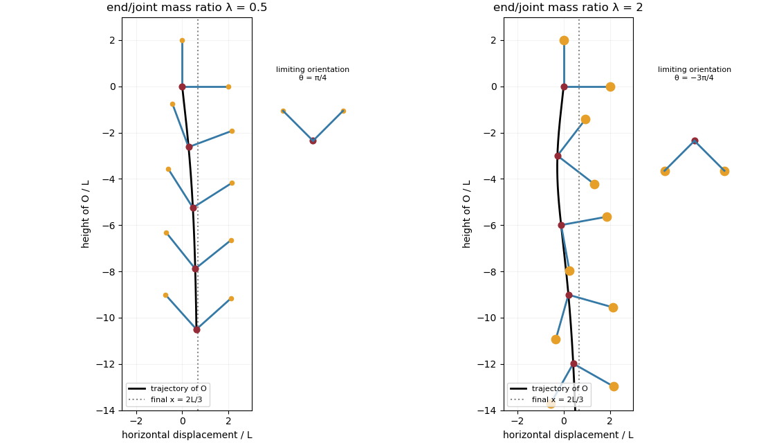
Take laboratory vertical velocity positive upwards. The body axes are $e_1=(\cos \theta ,\sin \theta )$ and $e_2=(-\sin \theta ,\cos \theta )$. In quasistatic sedimentation the force and torque exerted on the fluid equal the gravitational resultants on the body:The out-of-plane block is unforced, so its positive hydrodynamic resistance matrix gives $U_z={\Omega }_x={\Omega }_y=0$. Substitution in the planar hydrodynamic mobility matrix givesandFor $0\le \lambda <1$, this ordinary differential equation has positive right side on $0\le \theta <\pi /4$, with a stable zero at $\pi /4$. Uniqueness prevents crossing that equilibrium in finite time. For $\lambda >1$ the initial angular velocity is negative, and the stable equilibrium reached from zero is $-3\pi /4$. The heavier-end body turns clockwise through $3\pi /4$; it does not settle at $\pi /4$. More explicitly, with $K=(1-\lambda )mg/(4C{L}^2)$,where the continuous branch has $\theta -\pi /4\in (-\pi ,0)$. At $\lambda =1$, $\theta$ remains zero.

Transforming the translational velocity back to laboratory axes givesFor $\lambda \ne 1$, eliminate time between $U_h$ and the angular velocity:At either limiting orientation $\sin \theta =\cos \theta$. Thus both cases have the same net horizontal displacement,For $\lambda <1$ the drift is monotonically rightwards. For $\lambda >1$ it first moves left, reaching $x_O-x_O(0)=(2L/3)(1-\sqrt{2})$ at $\theta =-\pi /4$, then reverses. The total horizontal path length in this second case is $(2L/3)(2\sqrt{2}-1)$, whereas its net displacement is $2L/3$ rightwards. At $\lambda =1$ it falls vertically without rotation or drift; taking the infinite-time limit before $\lambda \to 1$ is consequently singular.

For the requested sedimentation drift of a weighted two-rod body sketch, a full parametric trajectory follows by also integrating $U_v/\dot{\theta }$. Put $\psi =\theta -\pi /4$ and set the initial height to zero:It tends to $-\infty$ in either case while $x_O$ tends to $2L/3$. At $\lambda <1$ both rods end pointing upwards from $O$ symmetrically; at $\lambda >1$ they end pointing downwards symmetrically. The asymptotic downward speed is $(1+2\lambda )mg/(3CL)$.

Use the well-mixed natural ventilation model for a distributed floor source. Let the building height be $H_b$, its volume be $\mathcal{V}$, its temperature excess be $\theta$, and the exterior mass density be $\rho$. Let ${\alpha }_T$ be the coefficient of thermal expansion, so reduced gravity is $g^{\prime }=g{\alpha }_T\theta$. Convert the total heat input $Q$ to the temperature-volume flux $\mathcal{H}=Q/(\rho c_p)$, where $c_p$ is specific heat capacity. If the quoted heat flux is per floor area, first multiply it by that area.

For effective opening area for pressure-driven ventilation, define the equal-opening hydraulic coefficient $K_A$ such that the signed throughflow $q$ obeys $q|q|=K_A\Pi$, with $\Pi$ the total driving pressure divided by mass density. In the effective-area convention of question 6, each opening has discharge $A\sqrt{\delta p/\rho }$, so $K_A=A^2/2$. The usual physical-area orifice law instead gives $K_A=C_d^2{A}^2$; that prefactor does not affect the stability conclusions.

Set $W=\Delta P/\rho >0$ and $G_T=g{\alpha }_T{H}_b$. Positive $q$ denotes entry at the floor and exit at the roof. hydrostatic pressure and wind combine to giveBecause the inflowing air is at exterior temperature in either direction, the heat budget isThe well-mixed ventilation temperature balance at steady state is thereforeAll roots must satisfy $\theta >0$ and their appropriate flow-direction inequality; squaring a pressure relation without imposing those conditions could add spurious branches.

The assisting case has a unique positive solution and it is stable. For opposing wind, define ${\theta }_w=W/G_T$. There is always one solution with $\theta >{\theta }_w$, a buoyancy-dominated upward flow. Below ${\theta }_w$, the heat-removal curve is $R(\theta )=\sqrt{K_A}\theta \sqrt{W-G_T\theta }$. It is zero at both endpoints, and its maximum occurs at $\theta =2{\theta }_w/3$:For $0<\mathcal{H}<R_{\max }$ there are two downward-flow roots as well as the upward-flow root. Equivalently, setting $y=G_T\theta /W$ and $\epsilon =G_T\mathcal{H}/(\sqrt{K_A}{W}^{3/2})$, the equilibrium curve isFor linear stability analysis of the opposing-wind ventilation bistability, linearize the heat budget: the eigenvalue is $-R^{\prime }(\theta )/\mathcal{V}$. The cooler downward root has $0<\theta <2{\theta }_w/3$ and $R^{\prime }>0$, so it is stable. The warmer downward root has $2{\theta }_w/3<\theta <{\theta }_w$ and $R^{\prime }<0$, so it is unstable and separates the two basins. The upward root has $R^{\prime }>0$ and is stable. At $\mathcal{H}=R_{\max }$ the two downward roots merge at a saddle-node bifurcation; above that value only the upward equilibrium remains.

For ventilation switching under wind and heating changes, increasing wind pressure or decreasing heat input both reduce $\epsilon$, so both can create the pair of wind-driven equilibria. They nevertheless have different physical and transient effects. On the hot upward branch, implicit differentiation of $\mathcal{H}=\sqrt{K_A}\theta \sqrt{G_T\theta -W}$ shows that increasing $W$ increases $\theta$, while decreasing $\mathcal{H}$ decreases $\theta$. Both reduce the upward ventilation rate, but only a wind change shifts ${\theta }_w$.

Under slow parameter variation, a state follows its current stable branch while that branch persists; the upward branch does not disappear when wind increases or heating decreases. A sufficiently large abrupt wind increase can raise ${\theta }_w$ beyond the current temperature and place that state below the new unstable threshold, causing flow reversal and cooling towards the wind-dominated equilibrium. A jump insufficient to cross its basin boundary returns to the upward equilibrium.

At fixed $W$, reducing a still-positive heat input cannot force an initially upward-flow state through ${\theta }_w$: at that boundary the temperature balance has $\dot{\theta }=\mathcal{H}/\mathcal{V}>0$. Thus heat reduction alone does not cause that reversal in this model. Conversely, decreasing wind or increasing heat from the stable downward branch eventually destroys it at the fold and forces a switch to the upward branch, giving history dependence. Wind strengthening and heat reduction have the same effect on the steady dimensionless control parameter, but not the same temperature change or switching dynamics. These stability statements use quasi-steady opening flow and a single well-mixed temperature; other stratification or airflow-inertia models require their own stability analysis.

Let $q_b$ be floor inflow and $q_t$ roof outflow. Use effective-area discharge $A\sqrt{\delta p/\rho }$, matching the factors in the supplied relations. With negligible source volume, both equal $q$. The lower region has exterior mass density while the warm upper layer has reduced gravity $g^{\prime }$ and depth $H-h$. hydrostatic pressure therefore supplies a total opening pressure head $g^{\prime }(H-h)$. Equal openings sharing equal discharge take half each, givingSteady lower-layer volume conservation sets this ventilation rate equal to the entrained turbulent plume flux at the interface, $q=\lambda B^{1/3}{h}^{5/3}$. Upper-layer buoyancy conservation gives $B=q{g}^{\prime }$. These are the required balances for displacement ventilation:Eliminating $g^{\prime }$ and $q$ gives the displacement-ventilation interface height equationThe left side is strictly increasing from zero to infinity, so there is one interface height. It depends on opening geometry and plume entrainment, not on $B$; the resulting $g^{\prime }=B^{2/3}/(\lambda h^{5/3})$ and throughflow do depend on $B$.

For finite source volume $Q$, conservation instead gives $q_t=q_b+Q$. The two pressure drops are no longer equal:Let $q_p(h;Q)$ be a physically entraining source plume: $q_p(0;Q)=Q$ and $q_p(h;Q)>Q$ for $h>0$. Its interface balance is $q_p=q_t=Q+q_b$. Therefore, as $q_b$ reaches zero, a positive-depth lower layer has no replenishment and cannot remain steady: this is no steady displacement layer without ambient supply. The limiting interface is $h=0$. At the threshold $q_t=Q$ and $g^{\prime }=B/Q$, and the entire hydrostatic head drives the roof discharge. HenceThis is source-volume blocking of displacement ventilation. The half-head factor of the negligible-source state must not be kept after the floor inflow vanishes. In the usual physical-area convention $q=A_{\mathrm{phys}}{C}_d\sqrt{2\delta p/\rho }$, the equivalent formula is $Q_c=(2C_d^2{A}_{\mathrm{phys}}^{2}BH{)}^{1/3}$.

The quoted pure-plume law cannot be used unmodified down to the origin for a source with nonzero volume: it would incorrectly give zero flux there. A compatible finite-source example uses a virtual origin,It recovers the supplied pure-plume limit when $Q\to 0$, and gives the same blocking threshold. The complete finite-$Q$ interface trajectory depends on that plume model, but the threshold needs only source-volume conservation and positive entrainment. For $Q>Q_c$, the assumed steady regime with a lower inflow no longer exists.

Write $\alpha =\Omega {\tau }_0^{\ast }$ and $s=\sin \theta$, where ${\tau }_0^{\ast }=t-R/c_0$. Label the two arms by $\sigma =\pm 1$. Their positions are $y_{\sigma }=\sigma r{e}_r(\Omega {\tau }_{\sigma }^{\ast })$. To radiating far-field accuracy,The retarded time equation therefore gives, with ${\mu }_r=\Omega r/c_0$,For the first arm, $\sigma =1$, this is the requested phase expansion. The more explicit geometric error also makes the dimensional meaning of the printed $O(1/R)$ term clear.

Apply the Taylor theorem to the rotating line force. Since $d{e}_{\varphi }/d\alpha =-e_r$, its first two orders, expressed in a common reference frame, areAlso $v_{\sigma }=\sigma \Omega r{e}_{\varphi }(\Omega {\tau }_{\sigma }^{\ast })$, so the radial Mach number isThe absolute value causes no change of sign in this subsonic limit. Multiplying these two expansions before summing is essential: both the shifted force and the moving-surface retarded Jacobian contribute at the same order.

Denote the integrated numerator, including that Jacobian, by $\mathcal{B}$. Pairing the two blades cancels all terms odd in $\sigma$, including the first Doppler correction to the axial load. HenceThe factor $a/3$ comes from $a^{-2}{\int }_0^a{r}^{2}dr$. Only the time-dependent term radiates at order $R^{-1}$. Applying $-{\partial }_{x_i}$ to the integral now gives ${\rho }_{\mathrm{rad}}^{\prime }=(4\pi c_0^{3}R{)}^{-1}n\cdot {\partial }_t\mathcal{B}$, and thusThere are also nonradiating terms of order $R^{-2}$. Multiply by $c_0^2$ for the acoustic pressure. The stated coefficient uses the rotation convention fixed above; reversing the rotation reverses the corresponding signed load and phase convention.

This is a compact rotating two-blade loading source acting as an acoustic quadrupole. The compact total rotating force cancels, leaving the first spatial moment of the loading. Its two factors of the observer's projection into the rotor plane produce ${\sin }^2\theta$: there is no leading sound on the rotation axis and the density amplitude is maximal in the rotor plane. The configuration repeats after half a rotation, explaining frequency $2\Omega$. These statements concern amplitude; the corresponding acoustic intensity has a ${\sin }^4\theta$ factor.

If $F=0$, the displayed first-order contribution vanishes as well. For completeness, expanding the axial Jacobian to its next even order givesThe first remaining axial-load radiation is thenThus the constant axial total force does not produce the lower-order term, even though its moving spatial distribution can radiate at a higher order.

Use the prescribed harmonic convention $e^{i\omega t}$. For a propagating acoustic plane wave, let $k=(\omega /c_0)\cos \theta$ and $\ell =(\omega /c_0)\sin \theta >0$. The incident and reflected pressure amplitudes in the upper half-space have vertical factors $e^{i\ell y}$ and $e^{-i\ell y}$ respectively:The linear homentropic acoustic equations imply $i\omega {\rho }_0{v}_y=-{\partial }_y{p}^{\prime }$. At the surface, the normal velocity is therefore $\ell (R-A)/({\rho }_0\omega )=-V$, while the pressure amplitude is $P=A+R$. The surface acoustic impedance condition $P=ZV$ givesHere $Z_f$ is the normal acoustic impedance; the angle in this question is measured from the horizontal, not the normal. For a passive acoustic impedance, the mean power absorbed per unit area is $\frac{1}{2}\mathrm{Re}(P{V}^{\ast })=\frac{1}{2}\mathrm{Re}Z|V{|}^2\ge 0$. The four limiting cases have distinct meanings:

Define $k_0=\omega /c_0$ and use the outgoing acoustic square-root branchFor positive real frequency reached from below, $\gamma =i\sqrt{k_0^2-k^2}$ on the propagating interval and is positive real for $|k|>k_0$. The outgoing field in the lower fluid has pressure amplitude $B{e}^{\gamma y}$, since $y<0$. If $\eta =\hat{\eta }{e}^{i\omega t-ikx}$, the shared normal velocity is $i\omega \hat{\eta }$. The linear homentropic acoustic equations therefore giveThis lower-fluid wave is outgoing; no additional incoming sound is included in defining the impedance seen by the upper fluid.

Put $K_s=T{k}^2-m{\omega }^2$. The sheet's force balance gives $K_s\hat{\eta }=-P+B$, hence $P=({\rho }_0{\omega }^2/\gamma -K_s)\hat{\eta }$. Its prescribed downward velocity amplitude is $V=-i\omega \hat{\eta }$. Thus the tensioned-sheet acoustic impedance isThe first term is the lower fluid's normal acoustic impedance, and the second is the sheet's inertial and elastic-sheet tension response. For a real propagating angle, $Z_f={\rho }_0{c}_0/\sin \theta$.

At fixed nonzero frequency and fixed wavenumber, $m\to \infty$ gives $|Z|\to \infty$, a zero-velocity, in-phase reflecting boundary. At fixed $k\ne 0$, $T\to \infty$ gives the same reflection limit, but there is an important exception: elastic-sheet tension does not resist the spatially uniform mode $k=0$. At normal incidence, the impedance remains ${\rho }_0{c}_0+im\omega$ however large the elastic-sheet tension is. With $m=0$ this mode is transparent. By contrast, arbitrarily large mass resists even a spatially uniform oscillation. These fixed-frequency limits exclude a simultaneously tuned structural resonance.

If $m=T=0$, $Z=Z_f$ and $R=0$. The identical fluids are effectively joined across a massless, untensioned interface: pressure and normal velocity continue without reflection. This is the matched case, rather than the pressure-release case.