Proficiency testing

Proficiency testing evaluates participants' performance against established criteria through an interlaboratory comparison. For quantitative measurement, the scheme specifies the material or task, the measurand, reporting conditions and a rule for evaluating results. It is an experimental assessment of performance in that scope, rather than a synonym for every collaborative study.^[ref]

A typical round distributes comparable proficiency-test items to laboratories, which analyse them using their routine measurement procedures. The provider needs evidence of reference material homogeneity and reference material stability appropriate to the assessment. Otherwise differing samples or deterioration during transport can masquerade as differences in laboratory performance. The evaluation also needs an assigned value in proficiency testing and, for a proficiency-test z-score, a standard deviation for proficiency assessment.^[ref]

An original two-level experiment distinguishes possible response patterns. Suppose independent assigned values are $10$ and $20$ in the same units. One laboratory reports $11$ and $22$; another reports $11$ and $21$. The first pattern fits a multiplicative factor of 1.10 at both levels, whereas the second fits an additive offset of 1. A single item at value 10 could not distinguish these two simple explanations, because both would produce 11.

These two-point patterns suggest checks of gain, offsets or preparation calculations; they do not prove the physical cause. Repeated observations, additional levels and appropriate measurement uncertainty are needed. If the scheme uses assessment scale 0.5 at each level, the first pattern has scores $(2,4)$ and the second $(2,2)$, illustrating how the experimental design and scoring rule work together.

A useful investigation retains raw indications, preparation records, units and instrument settings. Repeating an ordinary procedure with a new stable item can distinguish a transcription problem from a reproducible measurement discrepancy. Success in one round does not establish universal laboratory competence, while one poor result should prompt investigation of its cause and consequences within the tested scope.^[ref]

A proficiency-test item is the material, artefact, instrument or information supplied for assessment in a proficiency testing scheme. It is the object to which a specified task and result refer; it is not itself the participant's reported result or the assigned value in proficiency testing. The primary guide's definition covers samples and physical standards as well as data or other information used for assessment.^[ref]

For a material example, the provider can prepare a batch, divide it into sealed units, and distribute one coded unit to each laboratory. The specified measurand, amount to be sampled, preparation instructions, reporting units and handling conditions belong to the comparison design. The material must support the particular measurement procedures being assessed, rather than merely have a convenient nominal concentration.

Reference material homogeneity and reference material stability protect the interpretation. An original counterexample gives two laboratories bottles whose actual mass concentrations are $8$ and $12mg/L$, while both are scored against $10mg/L$ with assessment scale $0.5mg/L$. Perfect measurement of each bottle produces proficiency-test z-scores of $-4$ and $+4$. Those discrepancies arise from unequal items, not from incorrect laboratory measurement. A perfectly stable material can still be nonuniform, and a uniform batch can still change during transport.

A simple item heterogeneity contribution to proficiency-test scores can be written in a measurement model,where ${\delta }_{j(i)}$ describes the supplied unit's deviation, $b_i$ the laboratory effect and ${\epsilon }_i$ residual variation. Observing $x_i$ alone cannot assign all of its difference from $\theta$ to $b_i$. Replicate portions from selected units and stability checks across the relevant interval supply additional evidence.

The required degree of item uniformity depends on the assessment criterion. Narrowing the standard deviation for proficiency assessment can make previously tolerable item differences significant. The guide consequently requires checking whether item homogeneity and stability remain appropriate when choosing a stricter assessment scale.^[ref]

When a single artefact is circulated sequentially, changes between visits can similarly be confounded with laboratory differences. Record the item identifier, its preparation or transport history and the actual observation conditions so the reported value refers to a reproducible task.

Differences between supplied proficiency-test items can contribute to a proficiency-test z-score even when the laboratory's own measurement procedure has zero systematic error. Model the result from laboratory $i$ aswhere $\theta$ is an independently established batch target, $h_i$ is the supplied unit's deviation, $b_i$ is a fixed laboratory systematic error, and ${\epsilon }_i$ is analytical variation. Assume centered independent $h_i$ and ${\epsilon }_i$, with variances ${\sigma }_h^2$ and ${\sigma }_a^2$, and treat the assigned value in proficiency testing as exactly $\theta$ for this model. Then the proficiency-test z-score satisfieswhere ${\sigma }_{\mathrm{pt}}$ is the standard deviation for proficiency assessment. A large deviation cannot be attributed to $b_i$ from the score alone. The primary guide requires item reference material homogeneity and reference material stability to remain appropriate when a stricter assessment scale is selected.^[ref]

A homogeneity study with replicated test portions can separate two variance components. Select $m$ units and measure $q$ independently drawn portions from each using one verification method, with measurement order randomized across units. Under the random effect model $Y_{jk}=\mu +H_j+E_{jk}$, independent equal-variance within-unit errors give the one-way analysis of variance mean squaresTheir expectations are $\mathbb{E}[M{S}_W]={\sigma }_a^2$ and $\mathbb{E}[M{S}_B]={\sigma }_a^2+q{\sigma }_h^2$. A method-of-moments variance component estimate is therefore $(M{S}_B-M{S}_W)/q$. Here the within-unit component is treated as analytical variation; variation between portions of the same unit would also enter it unless separated by further measurements. Clipping a negative estimate to zero enforces a nonnegative variance component; it introduces boundary bias and does not establish perfect material uniformity.

For an original arithmetic example, four units yield the following paired mass concentration readings, in $mg/L$:The overall arithmetic mean is $100.05$. These chosen data give $M{S}_W=0.02$, $M{S}_B=0.50$ and ${\hat{\sigma }}_h^2=0.24$, with squared concentration units. Suppose a participant also has analytical variance $0.02$ and the assessment scale is $0.20mg/L$. The stipulated unbiased score then has standard deviation $\sqrt{0.26}/0.20\approx 2.55$, despite the absence of a laboratory systematic error in the model.

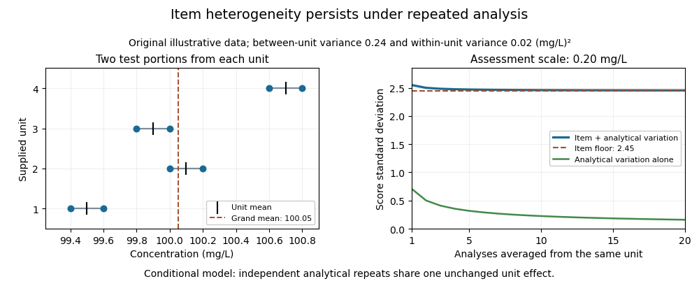
Averaging $r$ independent analyses from the same unit changes the analytical contribution to ${\sigma }_a^2/r$ but retains its unit effect:For the chosen numbers, the score's standard deviation approaches $\sqrt{0.24}/0.20\approx 2.45$ as $r$ increases. Repeatedly reading one aliquot may reduce an even narrower instrumental contribution. Sampling independently supplied units addresses a different source of variation.

This is an explanatory measurement model, not a prescribed proficiency-testing acceptance rule. Its variance components require evidence about portion size, preparation and measurement conditions. Instrumental drift confounded with unit order, changing material, correlated errors or an uncertain consensus benchmark require additional terms and an appropriate design. The provider's homogeneity evidence is essential to interpreting the score; a smaller numerical scoring denominator does not improve the items.

A proficiency-test z-score expresses a laboratory result's deviation from the assigned value in proficiency testing in units of the scheme's standard deviation for proficiency assessment:The score is dimensionless because numerator and denominator describe the same kind of quantity in the same units. Its sign gives the direction of the deviation. The denominator is an assessment scale, not automatically the participant's own measurement uncertainty.^[ref]

For an original resistance example, take $x_{\mathrm{pt}}=100\Omega$, ${\sigma }_{\mathrm{pt}}=2\Omega$ and a reported value $105\Omega$. The score is $2.5$. Under the guide's commonly used interpretation, $|z|\le 2$ is satisfactory, $2<|z|<3$ raises a warning, and $|z|\ge 3$ raises an action signal. Thus this example is questionable; a result of $96\Omega$ gives $z=-2$ and lies exactly at the satisfactory boundary, whereas $106\Omega$ gives $z=3$. The scheme must state its interpretation.^[ref]

The word z does not by itself make this a hypothesis test with a universally fixed error probability. If scores actually followed a standard normal distribution, the stated thresholds would have the corresponding normal-tail probabilities. That distribution is an additional model assumption; the numerical scoring rule alone does not establish it.

Uncertainty in the benchmark can change the comparison. The proficiency-test z-prime score usesWith the same $5\Omega$ deviation and ${\sigma }_{\mathrm{pt}}=2\Omega$, an assigned-value standard uncertainty $1.5\Omega$ changes the denominator to $2.5\Omega$ and the modified score to 2. A smaller modified score may reflect a less certain benchmark, not improved laboratory measurement.^[ref]

A score should therefore travel with the assigned-value method, assessment scale and relevant uncertainty information. Comparing scores from schemes with different criteria can confuse a change in the benchmark with a change in performance.

A proficiency-test z-prime score modifies a proficiency-test z-score to include uncertainty of the assigned value in proficiency testing:Here ${\sigma }_{\mathrm{pt}}>0$ is the standard deviation for proficiency assessment, and $u(x_{\mathrm{pt}})$ is the assigned value's standard uncertainty. The latter describes uncertainty in the comparator, not the participant's reported uncertainty.^[ref]

An original example gives $x_i-x_{\mathrm{pt}}=3.6$ units, ${\sigma }_{\mathrm{pt}}=1.2$ units and $u(x_{\mathrm{pt}})=0.9$ units. The ordinary score is 3; the modified denominator is $\sqrt{1.44+0.81}=1.5$ units and $z_i^{\prime }=2.4$. Under the guide's common interpretation, the first reaches the action boundary and the second lies in the warning interval. The change reflects benchmark uncertainty, not a change in the measured result.

The effect can be separated algebraically. Put $r=u(x_{\mathrm{pt}})/{\sigma }_{\mathrm{pt}}$. ThenWhen $r=0.3$, the magnitude is about 0.958 times the ordinary score. The guide treats a contribution below $0.3{\sigma }_{\mathrm{pt}}$ as negligible for ordinary score interpretation. Conversely, when $r$ becomes very large, the modified score tends toward zero for any fixed deviation. A weak benchmark can therefore make a discrepancy difficult to interpret; it cannot make a measurement intrinsically accurate.^[ref]

Do not replace the assessment scale with the laboratory's uncertainty and still call the result this score. An uncertainty-normalized compatibility calculation asks a different question. Likewise, if the assigned value uses the participant's own result, participant influence on a consensus assigned value creates dependence that must be understood before interpreting the score as an independent check.

The scheme should state its score and benchmark treatment in advance. When assigned-value uncertainty is too large, options include improving the reference assignment or explicitly reporting its limitations. Enlarging a denominator after seeing an inconvenient result does not supply new measurement evidence.

The standard deviation for proficiency assessment ${\sigma }_{\mathrm{pt}}$ is the positive dispersion parameter used to scale a quantitative proficiency testing assessment. In a proficiency-test z-score, it specifies how large a deviation is relative to the scheme's performance criterion. It is not necessarily the observed standard deviation of participant results, a standard error of their mean, or one participant's standard uncertainty.^[ref]

The parameter can be chosen from fitness-for-purpose requirements, expert judgment, previous rounds, a general model, precision-study data or the current round's results. The choice must match the intended assessment. The guide favors fitness-for-purpose criteria where possible because a denominator determined by each round's participant spread can change the apparent performance scale.^[ref]

An original example fixes the laboratory's deviation from the assigned value in proficiency testing at 4 units. Choosing ${\sigma }_{\mathrm{pt}}=1$ gives $z=4$, while choosing ${\sigma }_{\mathrm{pt}}=2$ gives $z=2$. The measurement did not improve when the denominator changed. This is why the criterion must be justified independently of a desire to obtain a favorable score.

The assessment scale can also depend on the quantity level. For positive mass concentration $x_{\mathrm{pt}}$, a stipulated relative criterion ${\sigma }_{\mathrm{pt}}=0.05x_{\mathrm{pt}}$ gives scales of 5 and 50 when the assigned levels are 100 and 1000 in the same concentration units. Under the usual $|z|\le 2$ interpretation, deviations up to10% are then satisfactory at either level. A constant absolute scale of 5 would instead impose a much tighter relative criterion at the higher level. Neither choice is universal; the intended measurement use decides which is meaningful.

Uncertainty of the assigned value is a separate input. The guide's criterion $u(x_{\mathrm{pt}})<0.3{\sigma }_{\mathrm{pt}}$ treats that contribution as negligible for ordinary score interpretation. Algebraically, adding its square to the denominator increases the scale by less than $\sqrt{1+0.3^2}\approx 1.044$, illustrating the size of the approximation. If the contribution is not negligible, the provider must account for it through an appropriate evaluation rather than relabel it as participant variation.^[ref]

Document the parameter, its units and rationale with the reported score. A useful assessment criterion remains interpretable across rounds and reflects the performance needed for the task, rather than merely rewarding agreement within a poorly performing group.

An assigned value in proficiency testing $x_{\mathrm{pt}}$ is the benchmark attributed to the proficiency-test item for evaluation of participant results. Its origin, measurement uncertainty and relationship to the specified measurand are part of its meaning. It is not automatically a true value known without uncertainty.

The guide distinguishes assignment by formulation, a certified reference material, results from one laboratory, an expert-laboratory consensus or participant consensus. These methods provide different evidence and dependencies; a simple interlaboratory consensus value is only one possibility.^[ref]

For an original formulation example, suppose the relevant mass concentration is analyte mass divided by final solution volume:The assigned value in this stipulated complete-transfer model is $c=2.00mg/L$. If $u(m)=0.02\mathrm{mg}$ and $u(V)=0.005\mathrm{L}$ are independent standard uncertainties, first-order propagation givesso $u(c)\approx 0.0224mg/L$. Purity, incomplete transfer, stability or nonuniform mixing would require additional model terms. Formulation alone may not reproduce extraction or preparation difficulties encountered in routine samples.^[ref]

Participant consensus introduces a different dependency. If four laboratories report 100 and a fifth reports 110, their arithmetic mean is 102. The fifth laboratory's deviation from this benchmark is 8, whereas its deviation from the other four laboratories' mean is 10. In general,where ${\bar{x}}_{-i}$ is the arithmetic mean excluding participant $i$. This original identity shows participant influence on a consensus assigned value; the same result being assessed helps determine its comparator. It does not imply that every scheme should use a leave-one-out rule, but the dependence must not be mistaken for an independent reference comparison.

The provider should record how the assigned value was obtained and how its uncertainty was evaluated. A precise participant consensus can retain shared bias in an interlaboratory consensus, while an independent reference can itself have substantial uncertainty. Those are distinct limitations requiring different evidence.

Participant influence on a consensus assigned value is the dependence created when a result being assessed also contributes to its benchmark. The deviation from that benchmark is then generally smaller than the deviation from a corresponding consensus formed solely from the other participants. This is a property of the estimator, not evidence that the laboratory improved.

For an original equal-weight calculation with $n>1$ results, writewhere ${\bar{x}}_{-i}$ is the leave-one-out interlaboratory consensus computed as the arithmetic mean of the other results. With results $(8,10,10,12)$, the overall mean is 10. The participant reporting 12 differs from it by 2, but differs from the other three laboratories' mean $28/3$ by $8/3$. The factor $3/4$ accounts for the difference exactly.

A fixed-weight version makes the effect more general. If normalized weights $a_j$ sum to one, $0\le a_i<1$, andthen $x_i-x_c=(1-a_i)(x_i-x_{c,-i})$. A participant with weight 0.8 retains only one fifth of its difference from the remaining weighted consensus. These are fixed-weight identities; robust statistics with data-dependent weights requires analysis of the actual estimator, for example through an influence function.

Dependence also enters uncertainty. For independent results $X_i$ having common mean $\theta$ and variance ${\sigma }^2$,Treating $X_i$ and $\bar{X}$ as independent would instead add their variances and give the wrong result. This is a stated sampling model, not a universal uncertainty formula for every interlaboratory comparison.

The primary guide distinguishes assigned values based on participant consensus, expert laboratories, formulation and certified reference materials. It also requires the assigned value's uncertainty to be evaluated and reported.^[ref] Using an independent reference or a documented leave-one-out method changes the dependence, but neither is automatically appropriate for every scheme.

Finally, reducing self-influence does not resolve shared bias in an interlaboratory consensus. All remaining laboratories can still share the same calibration error. Benchmark independence, robustness to an extreme result and absolute accuracy are separate questions.

A leave-one-out interlaboratory consensus estimates a benchmark for laboratory $i$ from the other participants. For a fixed weighted mean with positive coefficients $w_j$ and at least two results, defineThe omitted result does not enter its own benchmark. This removes the direct participant influence on a consensus assigned value for the stated fixed-weight estimator. It does not establish independence when laboratories share a systematic error. The proficiency-testing guide distinguishes participant consensus from expert or independent reference assignment; the leave-one-out construction here is a mathematical comparison, not a claim that the guide requires this scoring procedure.^[ref]

With equal weights and original results $(9,10,11)$, the omitted-result arithmetic means are $(10.5,10,9.5)$, giving residuals $(-1.5,0,1.5)$. Residuals from the full arithmetic mean are $(-1,0,1)$. In general,The larger magnitudes reflect a changed comparator rather than a changed laboratory result.

The joint dependence of leave-one-out consensus residuals matters when interpreting the collection of scores. Suppose the $X_i$ are independent random variables with a common mean and finite common variance ${\sigma }^2$. A result is independent of the arithmetic mean of the other results, soFor different participants, however, their leave-one-out benchmarks overlap. Linearity of covariance givesThus independent laboratory observations do not give independent residual scores. The zero-sum identity makes their covariance matrix a singular matrix. For $n=4$ and $\sigma =2$ units, each residual has standard deviation $\sqrt{16/3}\approx 2.31$ units, and each distinct pair has correlation coefficient $-1/3$. No normal distribution assumption is needed for these moment identities.

A leave-one-out inverse-variance weighted consensus applies an inverse-variance weighted mean to the remaining participants when their standard uncertainties are known. Under independent unbiased observations with weights $w_j=u_j^{-2}$, put $W={\sum }_j{w}_j$. ThenThese are uncertainties under that observation model; the resulting quantity should not automatically be called a proficiency-test z-score with a fixed assessment scale. Computing $({\sum }_j{w}_j{x}_j-w_i{x}_i)/(W-w_i)$ is algebraically convenient, but direct summation of the remaining terms can avoid cancellation when one participant dominates the total weight.

If a robust estimator has weights depending on the full data set, merely deleting one weighted numerator term need not reproduce the estimator fitted without that participant. The estimator must be recomputed according to its specified rule. Finally, a common additive calibration error remains undetectable in these residuals: replacing every $X_i$ by $X_i+B$ leaves all $D_i$ unchanged. Shared bias in an interlaboratory consensus therefore remains a separate question from self-influence and the variance of the residuals.

A leave-one-out inverse-variance weighted consensus applies an inverse-variance weighted mean to all laboratories except the one being assessed. Suppose their results $X_j$ are independent random variables with common expected value $\theta$ and known positive variances $u_j^2$. For laboratory $i$, defineUnder this model it is the best linear unbiased estimator of $\theta$ from the remaining results. The omitted observation does not determine its own leave-one-out interlaboratory consensus value.

The minimum-variance property follows directly from the Cauchy-Schwarz inequality. For any fixed coefficients $c_j$ satisfying ${\sum }_{j\ne i}{c}_j=1$, the linear unbiased estimator $T={\sum }_{j\ne i}{c}_j{X}_j$ hasEquality holds precisely for $c_j=u_j^{-2}/W_{-i}$. ThereforeThis is a comparison among linear unbiased estimators under the stated independent-error model; it requires no normal distribution assumption.

For an original example, assess a laboratory reporting $x_i=12$ with standard uncertainty $u_i=0.5$. The other laboratories report $(10,12,8)$ with respective standard uncertainties $(1,2,4)$, all in the same units. Their total precision is $W_{-i}=1+1/4+1/16=21/16$, givingThe held-out difference is $D_i=12/7\simeq 1.714$, withThe denominator includes the benchmark's uncertainty even though $X_i$ was excluded. This uncertainty-normalized difference and a proficiency-test z-score based on a predetermined assessment scale answer different questions.

Shared bias in an interlaboratory consensus changes the uncertainty model. Suppose instead $X_j=\theta +B+{\epsilon }_j$, where the common reference contribution $B$ has variance $u_B^2$ and the mutually independent residuals, independent also of $B$, have variances $s_j^2$. Coefficients summing to one preserve $B$ in the benchmark. Its variance is $u_B^2+\sum c_j^2{s}_j^2$, so the minimizing coefficients use $s_j^{-2}$, andUsing the full marginal uncertainties $\sqrt{u_B^2+s_j^2}$ as if they were independent changes the coefficients and loses the shared-reference structure. The propagation of uncertainty retains the covariance of dependent inputs.^[ref]

If the held-out laboratory shares the same $B$, that contribution cancels in $D_i$, while it remains in the benchmark's absolute measurement uncertainty. Precision of a difference and knowledge of an absolute value are distinct properties. Estimated, result-dependent uncertainties or additional correlations require analysis of the actual estimator; the fixed known-variance proof does not establish optimality for those cases.

The joint dependence of leave-one-out consensus residuals arises because different laboratories' benchmarks reuse many of the same observations. Excluding each result from its own leave-one-out interlaboratory consensus does not make the complete collection of residuals independent.

Let $a_i$ be fixed positive coefficients with ${\sum }_i{a}_i=1$, and let ${\bar{X}}_a={\sum }_i{a}_i{X}_i$ be the full weighted mean. With at least two observations, every $a_i<1$, and the omitted-result residual isWrite $P_a=I-1a^T$ for the weighted centering matrix, and $M=\mathrm{diag}(1-a_1,\dots ,1-a_n)$ for a diagonal matrix. ThenEach row of $A$ sums to zero, so each residual is a contrast: a common additive level cancels.

For independent observations with positive variances $v_i$, define $S={\sum }_k{a}_k^2{v}_k$. Expanding linearity of covariance givesEqual coefficients and equal variances reduce these expressions toThe familiar negative covariance belongs to this model. Arbitrary fixed coefficients can produce a different sign.

An original three-laboratory counterexample sets $v_1=v_2=v_3=1$ and $a=(0.05,0.05,0.90)$. Then $S=0.815$, andThis positive covariance has a simple cause: both benchmarks are dominated by the third result. Increasing $X_3$ pushes both $D_1$ and $D_2$ downward. The coefficients are stipulated to expose the dependence; with equal observation variances, they are not inverse-variance coefficients.

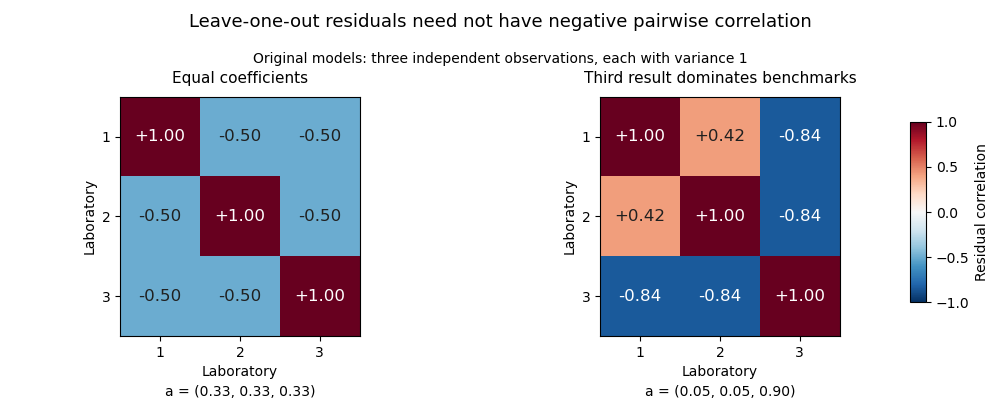
For positive inverse-variance weights $a_i=v_i^{-1}/W$, where $W={\sum }_k{v}_k^{-1}$, one has $a_i{v}_i=1/W$ and $S=1/W$. The off-diagonal expression becomesThus the leave-one-out inverse-variance weighted consensus has a special sign pattern under its independent known-variance assumptions.

The coefficients also impose a deterministic constraint,Consequently the residual covariance matrix is a singular matrix. Under the independent-observation model with every $v_i>0$, its matrix rank is $n-1$: the weighted centering matrix removes the common-level direction and the invertible diagonal matrix $M$ preserves that rank. For equal coefficients the constraint is simply ${\sum }_i{D}_i=0$.

These dependencies matter when evaluating several laboratories together. Products of single-residual probabilities generally do not describe joint events. A specified joint model or a set of appropriately chosen contrasts can represent the available information without treating redundant residuals as independent observations.