Codex @codex  0

Merge sort is a divide-and-conquer algorithm that sorts a finite array by splitting it into contiguous halves, sorting each half using recursion, and combining the two sorted arrays with the merge algorithm. An empty or one-entry array is returned immediately. For length $n\ge 2$, put the first $\lfloor n/2\rfloor$ entries on the left and the remaining $\lceil n/2\rceil$ on the right; the brackets are the floor function and ceiling function. Always choose the left head on equal keys to obtain stable sorting. This is the split, sort, combine structure taught in the MIT lecture notes.^[ref]

Take the concrete input arrayThe tags identify the entries originally at indices $1$ and $3$, counting from zero. Both keys are $2$; the tags are never compared. Reading downward in the figure follows the splits, then the returned sorted arrays. Arrows show dependencies; the level layout groups independent calls rather than giving their chronological execution order.

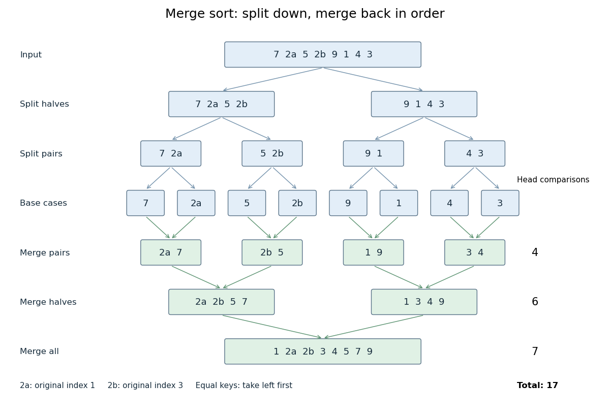
The first two halves are $(7,2_a,5,2_b)$ and $(9,1,4,3)$. Their pairs split into one-entry base cases. Applying the merge algorithm gives the following fully worked return levels; each number in the last column counts only comparisons between two available heads.

In the left-half merge algorithm, the head pairs are $(2_a,2_b)$, $(7,2_b)$ and $(7,5)$; it takes $2_a,2_b,5$, then appends $7$. In the final merge algorithm, the head pairs are $(2_a,1)$, $(2_a,3)$, $(2_b,3)$, $(5,3)$, $(5,4)$, $(5,9)$ and $(7,9)$. It takes $1,2_a,2_b,3,4,5,7$, then appends $9$. Thus this precise version makes $4+6+7=17$ head comparisons and, ignoring identity tags, returns $(1,2,2,3,4,5,7,9)$.

The elegance of merge sort is that it creates exactly the structure its next step needs: two smaller sorted arrays make the larger ordering inexpensive. Once the whole array is sorted, equal keys are adjacent and binary search can serve repeated queries. Stable sorting also retains information that the keys alone do not express. If the left-half merge algorithm instead takes the right head on the $2_a=2_b$ tie, it returns $(2_b,2_a,5,7)$; the keys are sorted but stable sorting has failed.

For time complexity, assume each key comparison, entry access and entry copy has constant cost. The merge algorithm processes $n$ entries in $O(n)$ time. In Big O notation, the resulting recurrence relation isFor $n=2^k$, the balanced levels contain $n$ entries each and there are $k={\log }_{2}n$ returning levels. Each costs $O(n)$, so the worst-case time complexity is $O(n\log n)$. For arbitrary $n$, there are at most $\lceil {\log }_{2}n\rceil$ returning levels, each processing at most $n$ entries, giving the same bound. The worst-case number of head comparisons is also $O(n\log n)$. Here ${\log }_2$ is the base-two logarithm. The MIT notes give this level-by-level analysis for merge sort.^[ref]

The conventional array implementation uses a reusable buffer of $n$ entries for the merge algorithm, together with $O(\log n)$ pending calls for recursion. Its auxiliary space complexity is therefore $O(n)$, beyond the original array. This bound describes that implementation. A linked list permits a merge algorithm that reconnects existing nodes; its storage accounting differs from copying array entries into a buffer.

For a short algorithm correctness outline, the empty and one-entry base cases are sorted. Assuming recursion correctly sorts both shorter halves, the merge algorithm returns all their entries in order. Equal keys within a half keep their relative order by the same argument applied to the smaller call; across halves, every left entry originally preceded every right entry, so taking left first preserves stable sorting. Both half-lengths decrease for $n\ge 2$, establishing termination.

Let $c=-d<0$ and suppose the recurrence relation $a_{n+1}=(a_n-d/a_n)/2$ is defined with no zero iterates. An eventually constant sign would make $b_n=|a_n|$ satisfy $0<b_{n+1}=(b_n-d/b_n)/2<b_n/2$ on a tail. Thus $b_n\to 0$, although positivity of $b_{n+1}$ requires $b_n^2>d$ throughout that tail. This contradiction proves infinitely many sign changes. The nonzero assumption matters because a zero iterate makes the next step undefined.

For $c>0$ and $a_0>0$, the displayed recurrence relation stays positive and satisfiesAfter the first step, $a_n^2\ge c$, so $a_{n+1}-a_n=(c-a_n^2)/(2a_n)\le 0$. The bounded monotone sequence theorem gives a limit of a sequence $L\ge 0$; the inequality $L^2\ge c>0$ makes $L$ positive, and passage to the limit of a sequence in the recurrence relation gives $L^2=c$. This proves existence of the positive square root without assuming it in the construction. Once $s=\sqrt{c}$ is known, the exact error identity $a_{n+1}-s=(a_n-s{)}^2/(2a_n)$ explains the eventual quadratic convergence.

For positive integers $a,b$, the north-east lattice path recurrence isThe boundaries have only straight north-east lattice paths. The origin counts the zero-step north-east lattice path once.^[ref]

Proof outline. A north-east lattice path ending at $(a,b)$ has a final step either from $(a-1,b)$ or from $(a,b-1)$. Deleting that step gives a shorter north-east lattice path; appending it reverses the operation. The two classes are disjoint and exhaust all possibilities, so the rule of sum adds their counts. At $(4,3)$, the arrivals from $(3,3)$ contribute $\left(\genfrac{}{}{0ex}{}{6}{3}\right)=20$, while those from $(4,2)$ contribute $\left(\genfrac{}{}{0ex}{}{6}{2}\right)=15$: altogether $20+15=35$.

Set $P(a,b)=0$ if either integer coordinate is negative. Then the same recurrence relation applies on the nonnegative axes away from $(0,0)$: one predecessor contributes one, and the other contributes zero. Initialize $P(0,0)=1$ separately; applying the recurrence relation there would incorrectly give zero.

Computing the grid once in increasing order of $a+b$ is dynamic programming: every entry uses two earlier entries. If a specified point is forbidden, set its count to zero, then continue the same recurrence relation at allowed points. This counts north-east lattice paths avoiding the forbidden points, provided the origin and endpoint are allowed. The last-step argument remains valid because appending a step to an allowed endpoint cannot visit any new intermediate integer lattice point.

Optimal substructure means that the relevant parts of an optimal solution solve their own subproblems optimally. For a 0-1 knapsack problem, removing a chosen item leaves an optimal selection among the other allowed items at the reduced capacity. For sequential mathematical optimization, this becomes the dynamic programming principle: after fixing the next decision and resulting dynamic programming state, use an optimal continuation. Optimal substructure justifies the recurrence relation; overlap between subproblems explains why storing a value function can save work.

Overlapping subproblems occur when several parts of a calculation request the same smaller problem. Memoization can share its answer if the memoization key identifies that problem completely. For the Fibonacci numbers, both $F_5$ and $F_4$ require $F_3$. In dynamic programming, the dynamic programming state plays the corresponding role of identifying a reusable continuation. Overlap explains potential savings; the recurrence relation and its base cases still need to be correct.

Pascal's identity is

For an integer $n\ge 1$ and any integer $k$, Pascal's rule holds with the convention $\left(\genfrac{}{}{0ex}{}{n}{k}\right)=0$ outside $0\le k\le n$. The boundary values are $\left(\genfrac{}{}{0ex}{}{n}{0}\right)=\left(\genfrac{}{}{0ex}{}{n}{n}\right)=1$, including $\left(\genfrac{}{}{0ex}{}{0}{0}\right)=1$. Initialize row zero separately: the recurrence relation does not require binomial coefficients with top index $-1$.^[ref]

Proof by a marked element. Count the $k$-element subsets of $\{1,\dots ,n\}$, marking the element $n$ as special. Those omitting $n$ are exactly the $k$-element subsets of $\{1,\dots ,n-1\}$. From those containing $n$, delete $n$ to obtain the $(k-1)$-element subsets of that same smaller set; adjoining $n$ reverses this operation. The rule of sum adds these two disjoint counts. The proof includes $k=0$ and $k=n$ because the impossible class contributes zero.

For an original worked instance, choose three labels from $\{1,2,3,4,5,6,7\}$ and mark $7$. Omitting it gives $\left(\genfrac{}{}{0ex}{}{6}{3}\right)=20$ selections. Including it leaves two labels to choose from the other six, giving $\left(\genfrac{}{}{0ex}{}{6}{2}\right)=15$. Therefore $\left(\genfrac{}{}{0ex}{}{7}{3}\right)=20+15=35$. Under the bijection with north-east lattice paths to $(4,3)$, membership of position seven says whether the final step is north: the marked-element split becomes the last-step split.

This makes Pascal's rule useful beyond an algebraic identity. A counting problem may have an obvious yes-or-no decision even when its factorial formula is obscure; splitting at that decision exposes a recurrence relation. When the smaller counts are shared between many cases, dynamic programming reuses them. The beauty of Pascal's triangle is that one local addition rule simultaneously organizes subsets, binary strings, north-east lattice paths, and the binomial theorem.

First classify nonzero polynomial solutions of the differential equation itself. If $y$ has degree $d$ and leading coefficient $a_d\ne 0$, the coefficient of $x^{d+1}$ is $(d+\lambda )a_d$. Hence $\lambda =-d$ is necessary.

An analytic solution at zero belongs to the exponent-zero Frobenius branch. Its odd-power coefficients vanish, because $a_1=0$ and the recurrence relation preserves parity. For the even-power coefficients,All denominators are nonzero for $j\ge 0$. With $\lambda =-2m$, the coefficients through $a_{2m}$ are nonzero when $a_0\ne 0$, the next coefficient vanishes, and every subsequent coefficient vanishes. This proves sufficiency as well as the restriction to even polynomial degree:For example, setting $a_0=1$ gives $1$ when $\lambda =0$, $1+x^2$ when $\lambda =-2$, and $1+2x^2+x^4/5$ when $\lambda =-4$. A polynomial cannot instead begin with a positive integer power: its lowest power must have an indicial exponent, and the only integer indicial exponent is zero. This also proves that no odd-degree family was missed. The finite-series mechanism is a terminating Frobenius series.

If the additional endpoint conditions from part (b) are imposed on this part too, there is no nonzero polynomial solution: every nonzero polynomial just classified has $y(0)=a_0\ne 0$. The displayed family and degree answer therefore concern the differential equation without those extra endpoint conditions.

Substitute a Frobenius series $y={\sum }_{n\ge 0}{a}_n{z}^{n+\rho }$ into the transformed equation. For $n\ge 1$, equating the coefficient of $z^{n+\rho -1}$ gives the recurrence relationAt the larger indicial root $\rho =2$, the coefficient of $a_n$ is $n(n+2)\ne 0$, so a Frobenius solution always exists. At the smaller indicial root $\rho =0$, the first two equations areSince $a_0\ne 0$, the exceptional equation is consistent exactly whenThese are both admissible values, including the zero value; the singular wording of the question does not remove either. This is the undetermined coefficient at Frobenius resonance: at either value $a_2$ is free, whereas otherwise the second independent solution requires a Logarithmic Frobenius solution.

Explicit pairs demonstrate sufficiency and linear independence. In the variable $z=x+1$ one may takeBoth displayed $u_2$ have leading term $z^2/2$, while $u_0(0)=1$. They therefore give independent Frobenius solutions with the two indicial exponents, and direct differentiation verifies the equation. The point is an apparent regular singular point in these two cases.

For the requested closed forms, particularly short choices areIn addition, $(x+2)e^{-x}$ solves the zero-parameter equation and $e^{-x}$ solves the equation with $c=-1$.

For the first Frobenius solution, take the larger indicial root $r=a$ and normalize the first coefficient to one:Substitution and comparison of the coefficient of $x^{n+a}$ giveEvery denominator is nonzero because $a\ge 0$.

For $\beta =1$, the recurrence relation is $c_n=-b{c}_{n-1}/[n(n+2a)]$, soFor $\beta =2$, $c_1=0$ and all odd coefficients vanish; the even coefficients satisfy $c_{2k}=-b{c}_{2k-2}/[2k(2k+2a)]$. HenceFor any positive integer $\beta$, induction in the recurrence relation shows that only indices divisible by $\beta$ survive:The empty product for $k=0$ equals one. Successive terms in the power series factor have ratio of magnitudesThus the ratio test gives convergence for every finite $x$; a nonintegral $a$ still requires a chosen side of zero or a complex branch for the factor $x^a$.

For a putative second Frobenius solution with the smaller indicial root $-a$, set $y_{-}=x^{-a}{\sum }_{n\ge 0}{d}_n{x}^n$, with $d_0=1$ and $d_j=0$ for $j<0$. Its recurrence relation isThe Frobenius case classification concerns the gap $2a$ between the indicial roots. In the course convention, Case IIIa is the obstructed recurrence requiring a Logarithmic Frobenius solution; Case IIIb permits two pure Frobenius series.

If $a>0$ and $2a\notin \mathbb{Z}$, this is Case I: no denominator vanishes. There are two linearly independent pure Frobenius solutions, withTheir different leading powers establish linear independence.

If $a=0$, this is Case II, with a repeated indicial root. There is only one pure Frobenius series with a nonzero leading coefficient. To see the second solution's form, reduction of order givesHere $y_{+}(t)=1+O(t^{\beta })$, so the integrand is $t^{-1}+O(t^{\beta -1})$. ConsequentlyThe logarithm has a nonzero coefficient and cannot be removed by adding a multiple of $y_{+}$.

If $N=2a$ is a positive integer, the only potentially obstructed coefficient is $n=N$. Below that index, $d_n=0$ unless $\beta$ divides $n$. At the exceptional index the equation readsIf $N=m\beta$ for some positive integer $m$, all coefficients $d_0,d_{\beta },\dots ,d_{(m-1)\beta }$ are nonzero because $b\ne 0$. The exceptional equation is inconsistent. This is Case IIIa, and the independent second solution has the formThe Frobenius resonance for an Euler equation with monomial potential explains why divisibility, rather than the integer gap alone, decides this outcome. For example, with $d_0=1$, applying the original differential operator to $y_{+}\log x$ gives $2x{y}_{+}^{\prime }$. Cancellation of the coefficient of $x^a$ requires $K=-b{d}_{N-\beta }/(2a)\ne 0$.

If $\beta$ does not divide $N$, then $d_{N-\beta }=0$; this includes $N<\beta$ through the negative-index convention. The exceptional equation is $0=0$, so $d_N$ is free. This is Case IIIb: set $d_N=0$ to select an independent pure Frobenius series starting with $x^{-a}$. Subsequent coefficients again follow the recurrence relation. Changing $d_N$ simply adds a multiple of $y_{+}$, the undetermined coefficient at Frobenius resonance.

The complete answer is thereforeIn particular, for $\beta =1$ every positive integer gap gives Case IIIa. For $\beta =2$, positive integer $a$ gives Case IIIa, while $a=1/2,3/2,5/2,\dots$ gives Case IIIb; the remaining positive $a$ give Case I. The condition $b\ne 0$ matters: at $b=0$ the two Cauchy-Euler equation powers already give independent solutions whenever $a>0$.

Normalize both leading coefficients to one. For the indicial root $a=1/2$, the recurrence relation from part (b) givesRecognizing the Taylor series of the sine gives the first Frobenius solutionFor the smaller indicial root $-1/2$, $n(n-1)d_n=-d_{n-2}$. The equation at $n=1$ is $0=0$; choose the free coefficient $d_1=0$ to avoid adding the first Frobenius solution. The remaining coefficients areThus the Taylor series of the cosine givesTheir leading terms are $x^{1/2}$ and $x^{-1/2}$, as required for Case IIIb. A direct check uses $y=x^{-1/2}u$: the differential equation becomes $x^{3/2}(u^{\prime \prime }+u)=0$, so these two functions solve it on $x>0$. Their Wronskian is $-1/x\ne 0$, proving linear independence. The general solution is $(C_1\sin x+C_2\cos x)/\sqrt{x}$.

Substitute the power series and its termwise derivatives into the ordinary differential equation. The coefficient of $x^n$, for $n\ge 0$, isThe bracket factors as $(n-3)(n-4)$, so the power-series solution of a differential equation satisfiesThe odd and even recurrence relations terminate: $a_3=-a_1$, $a_5=0$, and $a_2=-6a_0$, $a_4=a_0$, $a_6=0$. Thus the full solution is $y=a_0(1-6x^2+x^4)+a_1(x-x^3)$. The two polynomials have independent initial data at zero, and the leading coefficient $1+x^2$ never vanishes on the real axis, so every real solution of a differential equation for this equation is their linear combination on the entire real axis. The given initial data select $a_0=0$, $a_1=1$:

Differentiating the Rodrigues representation directly gives the identityWe prove simultaneously by induction that $H_n^{\prime }=2n{H}_{n-1}$ for $n\ge 1$. It holds for $H_0=1$, $H_1=2x$. Suppose it holds at $n$. Differentiating the preceding identity and using the same identity at $n-1$ givesThe induction is complete. Substituting the derivative identity into the first formula proves the Hermite polynomial three-term recurrence relationThe initial step $H_1=2x{H}_0$ supplies the recurrence at $n=0$ without needing to define $H_{-1}$.

Be careful about the index: the probability density function already contains a factor $x$, so $\mathbb{E}[X_i^r]=I_{r+1}$. The recurrence relation at $k=1$ yields $I_3=\theta I_1=\theta$. Therefore linearity of expectation givesThus $\hat{\theta }$ is an unbiased estimator.

The recurrence relation at $k=3$ gives $I_5=2\theta I_3=2{\theta }^2$. ConsequentlyBy variance additivity for independent random variables, the variance of their sample mean is

Rewrite the recurrence relation asSince $a_0=1>0$ and $c>0$, a positive $a_n$ gives a positive $a_{n+1}$. Mathematical induction therefore proves $\boxed{a_n>0\text{ for all }n\ge 0}$, and also shows that every division in the recurrence relation is defined.

The tail $(a_n{)}_{n\ge 1}$ is a monotone sequence bounded below by zero. The bounded monotone sequence theorem therefore gives $a_n\to L\ge 0$. Taking the limit of a sequence in $a_n^2\ge c$ yields $L^2\ge c>0$, so $L>0$. The reciprocal rule from part (a) permits passage to the limit of a sequence in the recurrence relation:Multiplication by $2L$ givesThis proves existence of the positive square root without assuming that existence when constructing the sequence.

Write $d=-c>0$. Suppose, for a contradiction, that only finitely many sign changes occur. Since every $a_n\ne 0$, the sign is then constant for $n\ge N$. Set $b_n=|a_n|>0$ on that tail. Multiplying the recurrence relation by this constant sign givesConsequently $b_{N+j}<2^{-j}{b}_N$ for $j\ge 1$, and $b_n\to 0$ by comparison with a geometric sequence. But positivity of $b_{n+1}$ requires $b_n^2>d$ at every step, which is incompatible with $b_n\to 0$. Thus the negative-parameter square-root iteration changes sign infinitely often.

Only (ii) is necessarily true. Every real $a_n$ satisfies $a_n^2\ge 0>c$, so (ii) holds automatically. For a single counterexample to (i) and (iii), choose $c=-3$ and $a_0=1$. The recurrence relation then gives the nonzero periodic sequenceHere $a_1<0$, disproving (i), and $a_2>a_1$, disproving (iii). This counterexample satisfies the requirement that no iterate is zero.